tidyTuesday meets the Economics of Majors
This week’s tidyTuesday focuses on degrees and majors and their deployment in the labor market. The original data came from 538. A description of sources and measures. The tidyTesday writeup is here.
library(tidyverse)
options(scipen=6)
library(extrafont)
font_import()
## Importing fonts may take a few minutes, depending on the number of fonts and the speed of the system.
## Continue? [y/n]Major.Employment <- read.csv("https://raw.githubusercontent.com/rfordatascience/tidytuesday/master/data/2018/2018-10-16/recent-grads.csv")
library(skimr)
skim(Major.Employment)| Name | Major.Employment |
| Number of rows | 173 |
| Number of columns | 21 |
| _______________________ | |
| Column type frequency: | |
| character | 2 |
| numeric | 19 |
| ________________________ | |
| Group variables | None |
Variable type: character
| skim_variable | n_missing | complete_rate | min | max | empty | n_unique | whitespace |
|---|---|---|---|---|---|---|---|
| Major | 0 | 1 | 5 | 65 | 0 | 173 | 0 |
| Major_category | 0 | 1 | 4 | 35 | 0 | 16 | 0 |
Variable type: numeric
| skim_variable | n_missing | complete_rate | mean | sd | p0 | p25 | p50 | p75 | p100 | hist |
|---|---|---|---|---|---|---|---|---|---|---|
| Rank | 0 | 1.00 | 87.00 | 50.08 | 1 | 44.00 | 87.00 | 130.00 | 173.00 | ▇▇▇▇▇ |
| Major_code | 0 | 1.00 | 3879.82 | 1687.75 | 1100 | 2403.00 | 3608.00 | 5503.00 | 6403.00 | ▃▇▅▃▇ |
| Total | 1 | 0.99 | 39370.08 | 63483.49 | 124 | 4549.75 | 15104.00 | 38909.75 | 393735.00 | ▇▁▁▁▁ |
| Men | 1 | 0.99 | 16723.41 | 28122.43 | 119 | 2177.50 | 5434.00 | 14631.00 | 173809.00 | ▇▁▁▁▁ |
| Women | 1 | 0.99 | 22646.67 | 41057.33 | 0 | 1778.25 | 8386.50 | 22553.75 | 307087.00 | ▇▁▁▁▁ |
| ShareWomen | 1 | 0.99 | 0.52 | 0.23 | 0 | 0.34 | 0.53 | 0.70 | 0.97 | ▂▆▆▇▃ |
| Sample_size | 0 | 1.00 | 356.08 | 618.36 | 2 | 39.00 | 130.00 | 338.00 | 4212.00 | ▇▁▁▁▁ |
| Employed | 0 | 1.00 | 31192.76 | 50675.00 | 0 | 3608.00 | 11797.00 | 31433.00 | 307933.00 | ▇▁▁▁▁ |
| Full_time | 0 | 1.00 | 26029.31 | 42869.66 | 111 | 3154.00 | 10048.00 | 25147.00 | 251540.00 | ▇▁▁▁▁ |
| Part_time | 0 | 1.00 | 8832.40 | 14648.18 | 0 | 1030.00 | 3299.00 | 9948.00 | 115172.00 | ▇▁▁▁▁ |
| Full_time_year_round | 0 | 1.00 | 19694.43 | 33160.94 | 111 | 2453.00 | 7413.00 | 16891.00 | 199897.00 | ▇▁▁▁▁ |
| Unemployed | 0 | 1.00 | 2416.33 | 4112.80 | 0 | 304.00 | 893.00 | 2393.00 | 28169.00 | ▇▁▁▁▁ |
| Unemployment_rate | 0 | 1.00 | 0.07 | 0.03 | 0 | 0.05 | 0.07 | 0.09 | 0.18 | ▂▇▆▁▁ |
| Median | 0 | 1.00 | 40151.45 | 11470.18 | 22000 | 33000.00 | 36000.00 | 45000.00 | 110000.00 | ▇▅▁▁▁ |
| P25th | 0 | 1.00 | 29501.45 | 9166.01 | 18500 | 24000.00 | 27000.00 | 33000.00 | 95000.00 | ▇▂▁▁▁ |
| P75th | 0 | 1.00 | 51494.22 | 14906.28 | 22000 | 42000.00 | 47000.00 | 60000.00 | 125000.00 | ▅▇▂▁▁ |
| College_jobs | 0 | 1.00 | 12322.64 | 21299.87 | 0 | 1675.00 | 4390.00 | 14444.00 | 151643.00 | ▇▁▁▁▁ |
| Non_college_jobs | 0 | 1.00 | 13284.50 | 23789.66 | 0 | 1591.00 | 4595.00 | 11783.00 | 148395.00 | ▇▁▁▁▁ |
| Low_wage_jobs | 0 | 1.00 | 3859.02 | 6945.00 | 0 | 340.00 | 1231.00 | 3466.00 | 48207.00 | ▇▁▁▁▁ |
A scatterplot of the unemployment rate by majors is the first goal with a color scheme that reflects the proportion of females in the industry.
my.plot <- Major.Employment %>% ggplot(aes(Unemployment_rate,Median, label=str_to_title(Major), color=ShareWomen)) +
  geom_point() +
  geom_text(check_overlap = T, vjust=-0.5, nudge_y=0.1, size=2.5) +
  theme_minimal() +
  scale_color_gradient(name="Share of Women", low="#de2d26", high = "#e9a3c9") +
  scale_y_continuous(labels = scales::comma) +
  scale_x_continuous(labels = scales::percent) +
  xlab("Unemployment Rate") +
  ylab("Median Income") +
  ggtitle("Median Income and Unemployment") +
  theme(text=element_text(size=8), title = element_text(size=12))
my.plot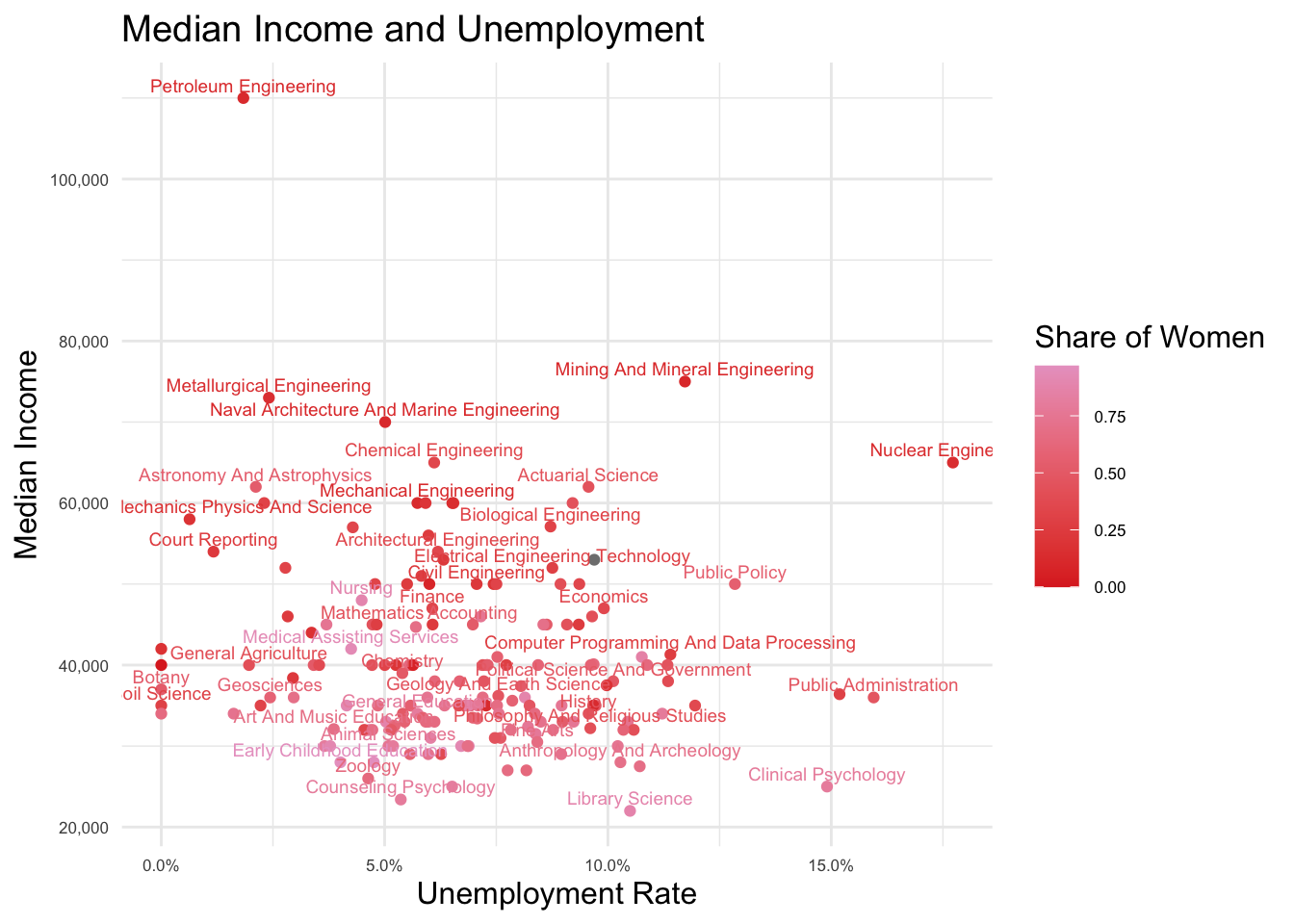
Major.Employment <- Major.Employment %>% mutate(ShareCol= College_jobs / Total)
my.plot <- Major.Employment %>% ggplot(aes(Unemployment_rate,ShareCol, label=str_to_title(Major), color=ShareWomen)) +
  geom_point(alpha=0.1) +
  geom_text(check_overlap = T, size=1.5) +
  theme_minimal() +
  scale_color_gradient(name="Share of Women", low="#de2d26", high = "#e9a3c9") +
#  scale_y_continuous(labels = scales::comma) +
  scale_x_continuous(labels = scales::percent) +
  xlab("Unemployment Rate") +
  ylab("College Pct.") +
  ggtitle("College Pct. Jobs and Unemployment")
my.plot
## Warning: Removed 1 rows containing missing values (geom_point).## Warning: Removed 1 rows containing missing values (geom_text).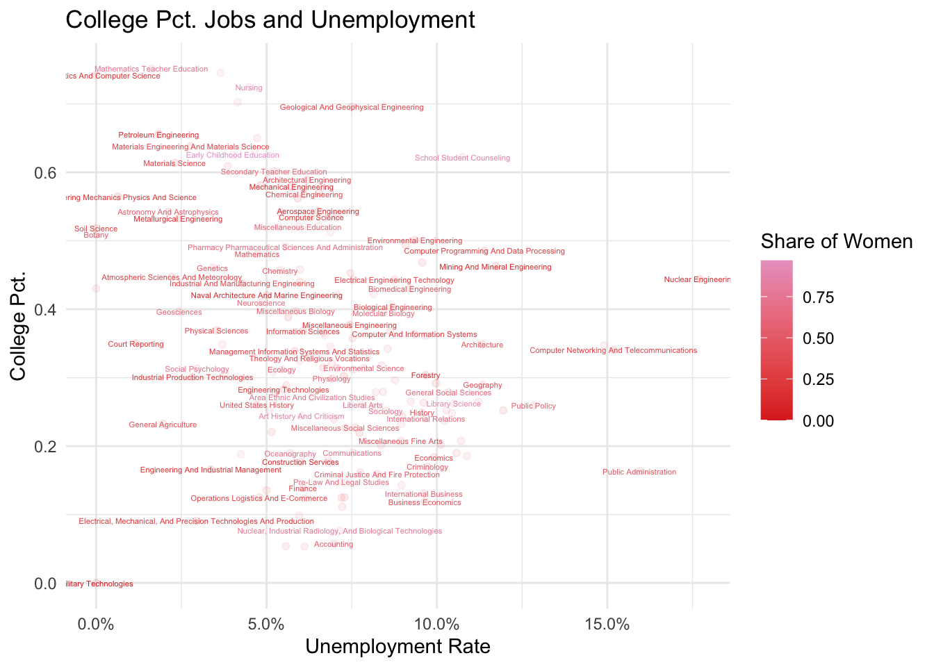
An Esquisse starter. Unemployment rate is x. Median wage is y. Major categories are colors and size is a function of Total
ggplot(data = Major.Employment) +
aes(x = Unemployment_rate, y = Median, color = Major_category, size = Total) +
geom_point() +
theme_minimal()
## Warning: Removed 1 rows containing missing values (geom_point).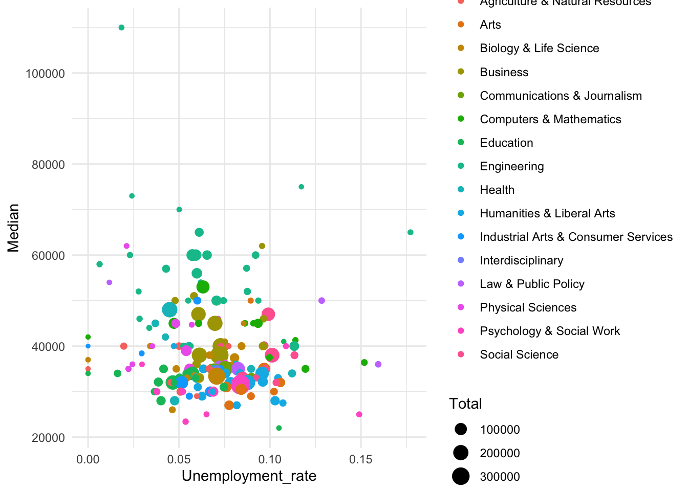
Major.Employment %>% drop_na() %>% ggplot() +
  aes(x = Unemployment_rate, y = Median, color = ShareWomen, label=str_to_title(Major)) +
#  geom_point() +
  geom_text(check_overlap = T, size=2) +
  theme_minimal() +
  scale_color_gradient(name="Share of Women", low="#cda7ca", high = "#3d323c") +
  scale_x_continuous(labels = scales::percent) +
  scale_y_continuous(labels = scales::comma) +
  xlab("Unemployment Rate") +
  ylab("Median Wage") +
  ggtitle("Wages and Unemployment with Women in the Profession")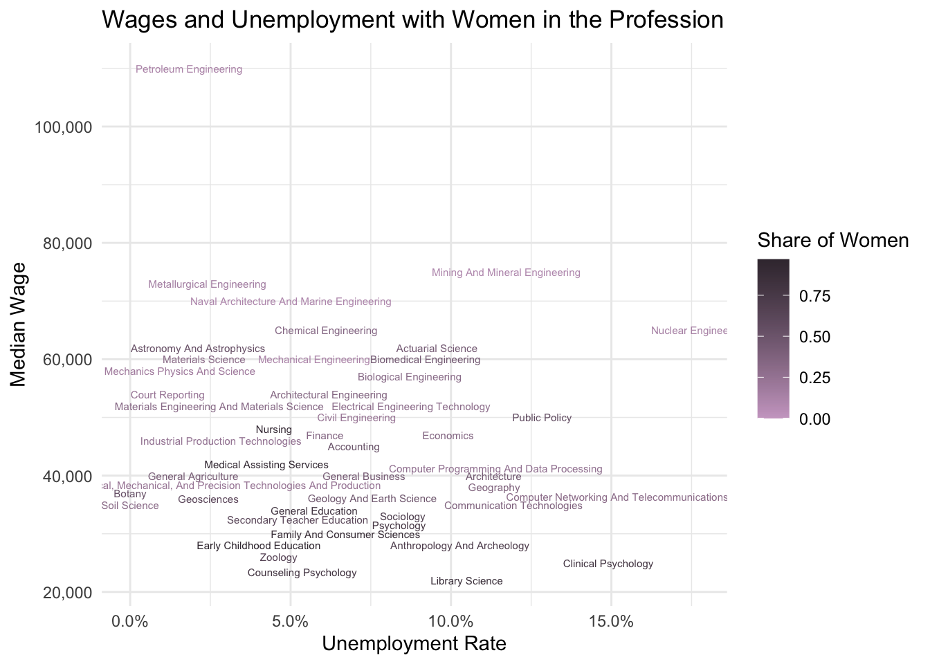
Alas.
Robert W. Walker
Associate Professor of Quantitative Methods
My research interests include causal inference, statistical computation and data visualization.