Spending on Kids
Spending on Kids
First, let me import the data.
kids <- read.csv('https://raw.githubusercontent.com/rfordatascience/tidytuesday/master/data/2020/2020-09-15/kids.csv')
# kids <- readr::read_csv('https://raw.githubusercontent.com/rfordatascience/tidytuesday/master/data/2020/2020-09-15/kids.csv')
Now let me summarise it and show a table of the variables.
summary(kids)## state variable year raw
## Length:23460 Length:23460 Min. :1997 Min. : -60139
## Class :character Class :character 1st Qu.:2002 1st Qu.: 71985
## Mode :character Mode :character Median :2006 Median : 252002
## Mean :2006 Mean : 1181359
## 3rd Qu.:2011 3rd Qu.: 836324
## Max. :2016 Max. :83666088
## NA's :102
## inf_adj inf_adj_perchild
## Min. : -60799 Min. :-0.01361
## 1st Qu.: 85876 1st Qu.: 0.12456
## Median : 298778 Median : 0.32757
## Mean : 1359983 Mean : 0.91448
## 3rd Qu.: 985049 3rd Qu.: 0.83362
## Max. :84584960 Max. :20.27326
## NA's :102 NA's :102A table of the variables. The definitions are best found here.
table(kids$variable)##
## addCC CTC edservs edsubs fedEITC
## 1020 1020 1020 1020 1020
## fedSSI HCD HeadStartPriv highered lib
## 1020 1020 1020 1020 1020
## Medicaid_CHIP other_health othercashserv parkrec pell
## 1020 1020 1020 1020 1020
## PK12ed pubhealth SNAP socsec stateEITC
## 1020 1020 1020 1020 1020
## TANFbasic unemp wcomp
## 1020 1020 1020It is very tidy. It is probably better shown after a pivot. 50 states, the District of Columbia, and 20 years gives us 1,020 observations. Let me show it wide.
Big.Wide <- pivot_wider(kids, id_cols = c(state,year), names_from = "variable", values_from = c("raw","inf_adj","inf_adj_perchild"))
Big.Wide
## # A tibble: 1,020 x 71
## state year raw_PK12ed raw_highered raw_edsubs raw_edservs raw_pell
## <chr> <int> <dbl> <dbl> <dbl> <dbl> <dbl>
## 1 Alab… 1997 3271969 956505 107733 246057 120833.
## 2 Alas… 1997 1042311 209433 5550 52355 7575.
## 3 Ariz… 1997 3388165 847032 111735 170281 120450.
## 4 Arka… 1997 1960613 457171 62447 189808 65904.
## 5 Cali… 1997 28708364 6858657 1121672 943805 775292.
## 6 Colo… 1997 3332994 861733 84129 77419 79004.
## 7 Conn… 1997 4014870 502177 71053 138932 36453.
## 8 Dela… 1997 776825 185114 31284 81880 9965.
## 9 Dist… 1997 544051 56693 0 0 18972.
## 10 Flor… 1997 11498394 2039186 391935 269777 318611.
## # … with 1,010 more rows, and 64 more variables: raw_HeadStartPriv <dbl>,
## # raw_TANFbasic <dbl>, raw_othercashserv <dbl>, raw_SNAP <dbl>,
## # raw_socsec <dbl>, raw_fedSSI <dbl>, raw_fedEITC <dbl>, raw_CTC <dbl>,
## # raw_addCC <dbl>, raw_stateEITC <dbl>, raw_unemp <dbl>, raw_wcomp <dbl>,
## # raw_Medicaid_CHIP <dbl>, raw_pubhealth <dbl>, raw_other_health <dbl>,
## # raw_HCD <dbl>, raw_lib <dbl>, raw_parkrec <dbl>, inf_adj_PK12ed <dbl>,
## # inf_adj_highered <dbl>, inf_adj_edsubs <dbl>, inf_adj_edservs <dbl>,
## # inf_adj_pell <dbl>, inf_adj_HeadStartPriv <dbl>, inf_adj_TANFbasic <dbl>,
## # inf_adj_othercashserv <dbl>, inf_adj_SNAP <dbl>, inf_adj_socsec <dbl>,
## # inf_adj_fedSSI <dbl>, inf_adj_fedEITC <dbl>, inf_adj_CTC <dbl>,
## # inf_adj_addCC <dbl>, inf_adj_stateEITC <dbl>, inf_adj_unemp <dbl>,
## # inf_adj_wcomp <dbl>, inf_adj_Medicaid_CHIP <dbl>, inf_adj_pubhealth <dbl>,
## # inf_adj_other_health <dbl>, inf_adj_HCD <dbl>, inf_adj_lib <dbl>,
## # inf_adj_parkrec <dbl>, inf_adj_perchild_PK12ed <dbl>,
## # inf_adj_perchild_highered <dbl>, inf_adj_perchild_edsubs <dbl>,
## # inf_adj_perchild_edservs <dbl>, inf_adj_perchild_pell <dbl>,
## # inf_adj_perchild_HeadStartPriv <dbl>, inf_adj_perchild_TANFbasic <dbl>,
## # inf_adj_perchild_othercashserv <dbl>, inf_adj_perchild_SNAP <dbl>,
## # inf_adj_perchild_socsec <dbl>, inf_adj_perchild_fedSSI <dbl>,
## # inf_adj_perchild_fedEITC <dbl>, inf_adj_perchild_CTC <dbl>,
## # inf_adj_perchild_addCC <dbl>, inf_adj_perchild_stateEITC <dbl>,
## # inf_adj_perchild_unemp <dbl>, inf_adj_perchild_wcomp <dbl>,
## # inf_adj_perchild_Medicaid_CHIP <dbl>, inf_adj_perchild_pubhealth <dbl>,
## # inf_adj_perchild_other_health <dbl>, inf_adj_perchild_HCD <dbl>,
## # inf_adj_perchild_lib <dbl>, inf_adj_perchild_parkrec <dbl>My brief plan
I recently came across a geofacet for R. I want to use it to plot a little bit of this data. If you want to get a head start, try install.packages("geofacet", dependencies=TRUE). You can google geofacet to get an idea of what a geofacet plot is. I will build one on the fly using a couple of tidy tools: filter, mutate, and joins and then put it together.
library(viridis)## Loading required package: viridisLitelibrary(geofacet)
state_ranks %>% filter(variable=="education") %>% select(state,name) -> mergeMe
p1 <- kids %>%
left_join(., mergeMe, by = c('state' = 'name')) %>%
filter(variable=="PK12ed")%>%
ggplot(., aes(x=year, y=inf_adj_perchild, color=inf_adj_perchild)) +
geom_line() +
facet_geo(~state.y) +
labs(x="year", y="Inflation Adjust Expenditures per child", title="Pre-K Through 12 Education Spending", color="Spend per child", caption="Data from #tidyTuesday: @PieRatio") +
scale_color_viridis_c() + theme_void()
p1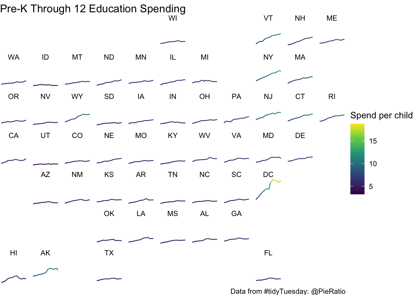
An Animation
library(gganimate)
p2 <- p1 + transition_reveal(year)
p3 <- animate(p2, renderer = gifski_renderer())
save_animation(p3, file = "./GeoAnimFacet.gif")
Animation
Neat-o an Oregon Grid
This isn’t very good though….
load(url("https://github.com/robertwwalker/rww-science/raw/master/content/R/COVID/data/OregonCOVID2020-09-15.RData"))
OR.County.COVID %>%
  mutate(County = str_replace(County, " ", "")) %>%
  ggplot(., aes(x=date, y=Number.of.cases, color=Number.of.cases)) +
  geom_line(size=1.5) +
  facet_geo(~ County, grid = "us_or_counties_grid1", label = "name", scales = "free_y") +
  scale_color_viridis_c(option = "plasma") +
  theme_void()
## Warning: Removed 3 row(s) containing missing values (geom_path).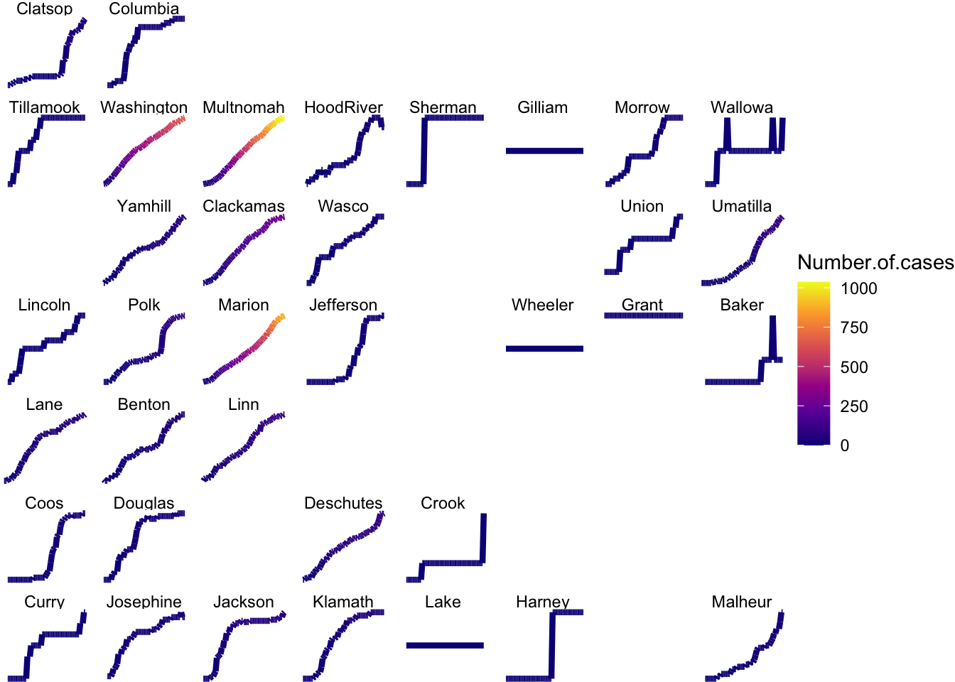
Robert W. Walker
Associate Professor of Quantitative Methods
My research interests include causal inference, statistical computation and data visualization.