Datasaurus Dozen
The datasaurus dozen
The datasaurus sozen is a fantastic teaching resource for examining the importance of data visualization. Let’s have a look.
datasaurus <- readr::read_csv('https://raw.githubusercontent.com/rfordatascience/tidytuesday/master/data/2020/2020-10-13/datasaurus.csv')##
## ── Column specification ────────────────────────────────────────────────────────
## cols(
## dataset = col_character(),
## x = col_double(),
## y = col_double()
## )Two libraries to make our work easy.
library(tidyverse)
library(skimr)
First, the summary statistics.
datasaurus %>% group_by(dataset) %>% skim()| Name | Piped data |
| Number of rows | 1846 |
| Number of columns | 3 |
| _______________________ | |
| Column type frequency: | |
| numeric | 2 |
| ________________________ | |
| Group variables | dataset |
Variable type: numeric
| skim_variable | dataset | n_missing | complete_rate | mean | sd | p0 | p25 | p50 | p75 | p100 | hist |
|---|---|---|---|---|---|---|---|---|---|---|---|
| x | away | 0 | 1 | 54.27 | 16.77 | 15.56 | 39.72 | 53.34 | 69.15 | 91.64 | ▁▇▃▇▁ |
| x | bullseye | 0 | 1 | 54.27 | 16.77 | 19.29 | 41.63 | 53.84 | 64.80 | 91.74 | ▂▆▇▅▂ |
| x | circle | 0 | 1 | 54.27 | 16.76 | 21.86 | 43.38 | 54.02 | 64.97 | 85.66 | ▅▃▇▅▃ |
| x | dino | 0 | 1 | 54.26 | 16.77 | 22.31 | 44.10 | 53.33 | 64.74 | 98.21 | ▅▇▇▅▂ |
| x | dots | 0 | 1 | 54.26 | 16.77 | 25.44 | 50.36 | 50.98 | 75.20 | 77.95 | ▂▁▇▁▅ |
| x | h_lines | 0 | 1 | 54.26 | 16.77 | 22.00 | 42.29 | 53.07 | 66.77 | 98.29 | ▅▇▇▅▁ |
| x | high_lines | 0 | 1 | 54.27 | 16.77 | 17.89 | 41.54 | 54.17 | 63.95 | 96.08 | ▂▅▇▃▁ |
| x | slant_down | 0 | 1 | 54.27 | 16.77 | 18.11 | 42.89 | 53.14 | 64.47 | 95.59 | ▂▅▇▃▁ |
| x | slant_up | 0 | 1 | 54.27 | 16.77 | 20.21 | 42.81 | 54.26 | 64.49 | 95.26 | ▃▆▇▃▂ |
| x | star | 0 | 1 | 54.27 | 16.77 | 27.02 | 41.03 | 56.53 | 68.71 | 86.44 | ▅▇▇▃▆ |
| x | v_lines | 0 | 1 | 54.27 | 16.77 | 30.45 | 49.96 | 50.36 | 69.50 | 89.50 | ▃▇▁▅▁ |
| x | wide_lines | 0 | 1 | 54.27 | 16.77 | 27.44 | 35.52 | 64.55 | 67.45 | 77.92 | ▇▂▁▇▅ |
| x | x_shape | 0 | 1 | 54.26 | 16.77 | 31.11 | 40.09 | 47.14 | 71.86 | 85.45 | ▇▆▁▃▅ |
| y | away | 0 | 1 | 47.83 | 26.94 | 0.02 | 24.63 | 47.54 | 71.80 | 97.48 | ▅▆▃▇▃ |
| y | bullseye | 0 | 1 | 47.83 | 26.94 | 9.69 | 26.24 | 47.38 | 72.53 | 85.88 | ▇▆▃▅▇ |
| y | circle | 0 | 1 | 47.84 | 26.93 | 16.33 | 18.35 | 51.03 | 77.78 | 85.58 | ▇▁▁▂▆ |
| y | dino | 0 | 1 | 47.83 | 26.94 | 2.95 | 25.29 | 46.03 | 68.53 | 99.49 | ▇▇▇▅▆ |
| y | dots | 0 | 1 | 47.84 | 26.93 | 15.77 | 17.11 | 51.30 | 82.88 | 94.25 | ▇▁▇▁▆ |
| y | h_lines | 0 | 1 | 47.83 | 26.94 | 10.46 | 30.48 | 50.47 | 70.35 | 90.46 | ▆▇▇▅▅ |
| y | high_lines | 0 | 1 | 47.84 | 26.94 | 14.91 | 22.92 | 32.50 | 75.94 | 87.15 | ▇▁▁▃▅ |
| y | slant_down | 0 | 1 | 47.84 | 26.94 | 0.30 | 27.84 | 46.40 | 68.44 | 99.64 | ▆▇▇▅▆ |
| y | slant_up | 0 | 1 | 47.83 | 26.94 | 5.65 | 24.76 | 45.29 | 70.86 | 99.58 | ▇▇▇▅▅ |
| y | star | 0 | 1 | 47.84 | 26.93 | 14.37 | 20.37 | 50.11 | 63.55 | 92.21 | ▇▂▂▅▅ |
| y | v_lines | 0 | 1 | 47.84 | 26.94 | 2.73 | 22.75 | 47.11 | 65.85 | 99.69 | ▇▆▇▃▅ |
| y | wide_lines | 0 | 1 | 47.83 | 26.94 | 0.22 | 24.35 | 46.28 | 67.57 | 99.28 | ▇▇▇▅▆ |
| y | x_shape | 0 | 1 | 47.84 | 26.93 | 4.58 | 23.47 | 39.88 | 73.61 | 97.84 | ▇▇▂▆▅ |
Notice that all of the datasets are nearly identical. But have a look at them.
datasaurus %>% ggplot() + aes(x=x, y=y, color=dataset) + geom_point() + facet_wrap(vars(dataset))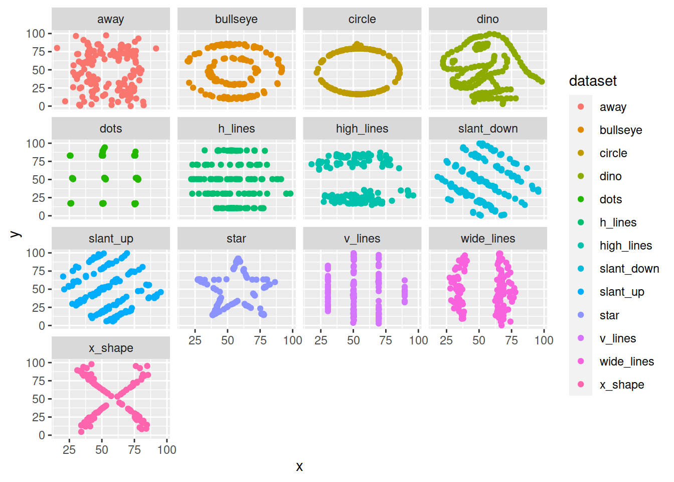
Robert W. Walker
Associate Professor of Quantitative Methods
My research interests include causal inference, statistical computation and data visualization.