Daily Weather Forecasting
Preliminary Steps
Load some libraries.
library(kableExtra)
library(distributional)
library(tidyverse)
library(lubridate)
library(hrbrthemes)
library(fpp3)
library(magrittr)
Loading NWS Data
Load the data.
# There is one blank variable name and some garbage at the top.  Skip the first
# six rows and label M and - as missing.
NWS <- read.csv(url("https://www.weather.gov/source/pqr/climate/webdata/Portland_dailyclimatedata.csv"),
    skip = 6, na.strings = c("M", "-")) %>%
    rename(Variable = X)
One thing that will prove troublesome is that /A appears in a few places. I want to remove it. I will ask R to find all of the character columns and remove /A.
NWS <- NWS %>%
    mutate(across(where(is.character), ~str_remove(.x, "/A")))
Let me produce the daily data.
NWS.Daily <- NWS %>%
    select(-AVG.or.Total)
names(NWS.Daily) <- c("YR", "MO", "Variable", paste0("Day.", 1:31))
NWS.Daily <- NWS.Daily %>%
    pivot_longer(., cols = starts_with("Day."), names_to = "Day", values_to = "value") %>%
    mutate(Day = str_remove(Day, "Day.")) %>%
    pivot_wider(., names_from = "Variable", values_from = "value") %>%
    mutate(PR = recode(PR, T = "O.005"), SN = recode(SN, T = "O.005")) %>%
    mutate(Temp.Max = as.numeric(TX), Temp.Min = as.numeric(TN), Precip = as.numeric(PR),
        Snow = as.numeric(SN), date = as.Date(paste(MO, Day, YR, sep = "-"), format = "%m-%d-%Y"))
NWS.Daily.Clean <- NWS.Daily %>%
    filter(!(is.na(date))) %>%
    filter(!is.na(TX)) %>%
    as_tsibble(index = date)
Data Evaluation
That nearly works. There are still a few missing values.
NWS.Daily.Clean <- NWS.Daily.Clean %>%
    filter(!is.na(Temp.Max))
NWS.Daily.Clean %>%
    tibble() %>%
    skimr::skim() %>%
    kable("html") %>%
scroll_box(width = "800px", height = "600px")| skim_type | skim_variable | n_missing | complete_rate | character.min | character.max | character.empty | character.n_unique | character.whitespace | Date.min | Date.max | Date.median | Date.n_unique | numeric.mean | numeric.sd | numeric.p0 | numeric.p25 | numeric.p50 | numeric.p75 | numeric.p100 | numeric.hist |
|---|---|---|---|---|---|---|---|---|---|---|---|---|---|---|---|---|---|---|---|---|
| character | Day | 0 | 1.0000000 | 1 | 2 | 0 | 31 | 0 | NA | NA | NA | NA | NA | NA | NA | NA | NA | NA | NA | NA |
| character | TX | 0 | 1.0000000 | 2 | 3 | 0 | 94 | 0 | NA | NA | NA | NA | NA | NA | NA | NA | NA | NA | NA | NA |
| character | TN | 0 | 1.0000000 | 1 | 2 | 0 | 73 | 0 | NA | NA | NA | NA | NA | NA | NA | NA | NA | NA | NA | NA |
| character | PR | 0 | 1.0000000 | 1 | 5 | 0 | 210 | 0 | NA | NA | NA | NA | NA | NA | NA | NA | NA | NA | NA | NA |
| character | SN | 0 | 1.0000000 | 1 | 5 | 0 | 59 | 1 | NA | NA | NA | NA | NA | NA | NA | NA | NA | NA | NA | NA |
| Date | date | 0 | 1.0000000 | NA | NA | NA | NA | NA | 1940-10-13 | 2019-12-31 | 1980-05-22 | 28934 | NA | NA | NA | NA | NA | NA | NA | NA |
| numeric | YR | 0 | 1.0000000 | NA | NA | NA | NA | NA | NA | NA | NA | NA | 1979.8894035 | 22.8684429 | 1940 | 1960 | 1980 | 2000.00 | 2019.00 | ▇▇▇▇▇ |
| numeric | MO | 0 | 1.0000000 | NA | NA | NA | NA | NA | NA | NA | NA | NA | 6.5358402 | 3.4527604 | 1 | 4 | 7 | 10.00 | 12.00 | ▇▅▅▅▇ |
| numeric | Temp.Max | 0 | 1.0000000 | NA | NA | NA | NA | NA | NA | NA | NA | NA | 62.6230386 | 14.4053209 | 14 | 52 | 61 | 73.00 | 107.00 | ▁▅▇▆▁ |
| numeric | Temp.Min | 0 | 1.0000000 | NA | NA | NA | NA | NA | NA | NA | NA | NA | 44.9852768 | 9.8193649 | -3 | 38 | 45 | 53.00 | 74.00 | ▁▁▇▇▁ |
| numeric | Precip | 3376 | 0.8833207 | NA | NA | NA | NA | NA | NA | NA | NA | NA | 0.1145172 | 0.2347028 | 0 | 0 | 0 | 0.13 | 2.69 | ▇▁▁▁▁ |
| numeric | Snow | 762 | 0.9736642 | NA | NA | NA | NA | NA | NA | NA | NA | NA | 0.0168572 | 0.2446811 | 0 | 0 | 0 | 0.00 | 14.40 | ▇▁▁▁▁ |
Snow and precipitation have missing values.
Daily Decompositions
I want to write a little function to decompose these data. It will take data and a variable of interest and decompose it. The trend and season windows are trendW and seasonW respectively.
Decompose.Me <- function(data, var, trendW = 5, seasonW = 5) {
    var <- ensym(var)
    model <- data %>%
        model(STL(!!var ~ trend(window = trendW) + season("week") + season("year")))
    cmp <- model %>%
        components()
    plot <- cmp %>%
        autoplot()
    return(list(model = model, cmp = cmp, plot = plot))
}
Let me look at Maximum Temperature.
MaxAvg.Result <- NWS.Daily.Clean %>%
    filter(YR > 1999) %>%
    Decompose.Me(., Temp.Max, trendW = 5)
MaxAvg.Result %>%
    .$plot
To work with the STL seasonally adjusted data, we can isolate season_adjust. This is the core component in STL+…
Let me decompose one such series. Suppose that I wanted to seasonally adjust this. I already have it there. season_7 is what I add to turn the season_adjust to the original.
MaxAvg.Result %>%
    .$cmp %>%
    head(10) %>%
    select(-.model)
# A tsibble: 10 x 7 [1D]
date Temp.Max trend season_week season_year remainder season_adjust
<date> <dbl> <dbl> <dbl> <dbl> <dbl> <dbl>
1 2000-01-01 46 64.7 -0.969 -18.9 1.10 65.8
2 2000-01-02 45 64.5 -0.274 -19.6 0.369 64.9
3 2000-01-03 45 63.9 -1.33 -16.5 -1.06 62.9
4 2000-01-04 50 63.3 1.14 -15.7 1.25 64.5
5 2000-01-05 47 62.0 0.949 -15.8 -0.214 61.8
6 2000-01-06 40 62.8 -0.443 -19.4 -2.90 59.8
7 2000-01-07 51 65.6 0.928 -17.9 2.39 68.0
8 2000-01-08 51 66.8 -0.997 -15.8 0.998 67.8
9 2000-01-09 48 63.9 -0.295 -15.9 0.214 64.2
10 2000-01-10 41 59.9 -1.32 -17.4 -0.167 59.7So let me run with that. Borrowing from an earlier post, I want a function to estimate models given data and an Outcome. It will have a few ARIMA with fourier terms and ARIMA, ETS, prophet.
Usual.Suspects <- function(data, Outcome) {
    Outcome <- ensym(Outcome)
    fits <- data %>%
        model(`K = 1` = ARIMA(!!Outcome ~ fourier(K = 1) + PDQ(0, 0, 0)), `K = 2` = ARIMA(!!Outcome ~
            fourier(K = 2) + PDQ(0, 0, 0)), `K = 3` = ARIMA(!!Outcome ~ fourier(K = 3) +
            PDQ(0, 0, 0)), ARIMA = ARIMA(!!Outcome), ETS = ETS(!!Outcome), NNET = NNETAR(!!Outcome ~
            fourier(K = 2)), prophet = prophet(!!Outcome ~ growth() + season(name = "annual"))) %>%
        mutate(Combo1 = (`K = 2` + ARIMA + ETS)/3, Combo2 = (`K = 2` + ARIMA + ETS +
            NNET)/4)
    return(fits)
}
Automagics
I want to write a magic function. It takes four inputs: data, Outcome, DateVar, and H.Horizon [defaults to 14]. The first one is the data. The next two inputs are Outcome, the outcome without quotation marks, and DateVar – the Date variable [the index of the tsibble], also unquoted. The final argument sets the forecast horizon [the plots will have two times this before them in real data from the test set]. I have tried to be copious in commenting this.
A Monthly Forecast Function
Accuse.Usual.Suspect <- function(data, Outcome, DateVar, H.Horizon = 14) {
    # Turn the symbols -- names that will make sense in their environments when
    # called -- that the user supplies into symbolics.  This is the role of ensym.
    Outcome <- ensym(Outcome)
    DateVar <- ensym(DateVar)
    # Create test using H.Horizon
    test <- data %>%
        slice_max(., order_by = !!DateVar, n = H.Horizon)  # Create train
    train <- data %>%
        anti_join(., test)
    # Estimate some models and store them as fits.  !! calls the variable name in the
    # given environment
    fits <- train %>%
        Usual.Suspects(., !!Outcome)
    # Forecast the models
    FC <- fits %>%
        forecast(h = H.Horizon)
    # Compare train and test using accuracy
    Accuracy.Table <- FC %>%
        accuracy(test)
    # Show the best fit
    Min.Model <- Accuracy.Table %>%
        slice_min(., order_by = MAE, n = 1)
    # Report on the best fitting model
    Min.Report <- fits %>%
        select(Min.Model$.model) %>%
        report()
    # Create a plot of the time series residuals for the best fit
    Min.Res.Plot <- fits %>%
        select(Min.Model$.model) %>%
        gg_tsresiduals()
    # Create a forecast plot for the best fitting model.
    Min.ForeCPlot <- FC %>%
        filter(.model == Min.Model$.model) %>%
        autoplot() + autolayer(test %>%
        select(!!Outcome)) + autolayer(data %>%
        slice_max(., order_by = !!DateVar, n = H.Horizon * 3) %>%
        select(!!Outcome)) + theme_ipsum_rc() + labs(title = "Winner Forecast")
    # Return a named list with all the stuff we calculated along the way.
    fit.list <- list(test = test, train = train, Model.Fits = fits, Model.Forecasts = FC,
        Accuracy.Table = Accuracy.Table, Min.Model = Min.Model, Min.Report = Min.Report,
        Min.Res.Plot = Min.Res.Plot, Min.Forecast.Plot = Min.ForeCPlot)
    return(fit.list)
}
Maximum Average Temperature
Try out the big function. Using all the data will be slow. Let’s try everything this century.
SAData <- MaxAvg.Result %>%
    .$cmp %>%
    select(-.model) %>%
    as_tsibble(index = date)
MaxAvg.Res <- SAData %>%
    Accuse.Usual.Suspect(., Outcome = season_adjust, DateVar = date, H.Horizon = 14)
Series: season_adjust
Model: NNAR(38,1,22)[7]
Average of 20 networks, each of which is
a 42-22-1 network with 969 weights
options were - linear output units
sigma^2 estimated as 5.798 What Won?
MaxAvg.Res$Min.Model# A tibble: 1 x 10
.model .type ME RMSE MAE MPE MAPE MASE RMSSE ACF1
<chr> <chr> <dbl> <dbl> <dbl> <dbl> <dbl> <dbl> <dbl> <dbl>
1 NNET Test 1.68 3.47 2.95 2.99 5.98 NaN NaN 0.327All the models on a 14 day horizon?
MaxAvg.Res$Accuracy.Table# A tibble: 9 x 10
.model .type ME RMSE MAE MPE MAPE MASE RMSSE ACF1
<chr> <chr> <dbl> <dbl> <dbl> <dbl> <dbl> <dbl> <dbl> <dbl>
1 ARIMA Test -0.987 4.54 3.84 -2.84 8.14 NaN NaN 0.531
2 Combo1 Test -1.04 4.53 3.76 -2.94 7.99 NaN NaN 0.547
3 Combo2 Test -0.376 4.04 3.23 -1.49 6.79 NaN NaN 0.506
4 ETS Test -0.0611 4.26 3.32 -0.878 6.93 NaN NaN 0.493
5 K = 1 Test -2.07 5.08 4.33 -5.11 9.30 NaN NaN 0.609
6 K = 2 Test -2.07 5.08 4.33 -5.11 9.29 NaN NaN 0.609
7 K = 3 Test -2.07 5.08 4.33 -5.11 9.29 NaN NaN 0.609
8 NNET Test 1.68 3.47 2.95 2.99 5.98 NaN NaN 0.327
9 prophet Test 2.84 5.00 4.04 5.22 8.05 NaN NaN 0.417Residuals?
MaxAvg.Res$Min.Res.Plot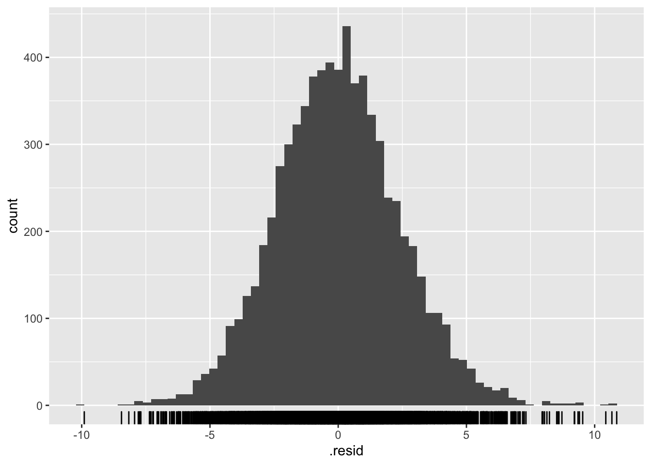
Try out a result.
MaxAvg.Res$Min.Forecast.Plot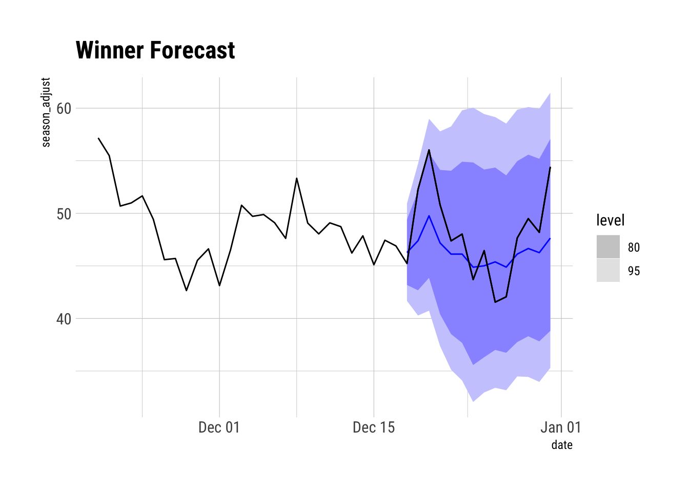
Robert W. Walker
Associate Professor of Quantitative Methods
My research interests include causal inference, statistical computation and data visualization.