TBATS for COVID-19 Data
Load the Previous Results for Comparison
Because this project was undertaken over more than one day, the live download of New York Times COVID-19 data will not necessarily match up. To sidestep this problem, I will load the data that I worked with previously.
load("data/AggForecast.RData")New Cases
First, I will manipulate the data to fit the old style of time series needed by TBATS.
# To use tbats, I need an old style time series First, select the data of
# interest: New.Cases and make it match up with the training set
NCT <- COVID.Agg.Train %>%
    filter(is_aggregated(state)) %>%
    select(New.Cases)
# Turn it into a time series.  Notice the axis is a mess
NCTS <- as.ts(NCT, frequency = 7)
NCTS
Time Series:
Start = 2020.24863387978
End = 2071.82006245121
Frequency = 7
[1] 26871 29673 32253 34952 25551 30875 30268 31634 34499 33395
[11] 31553 26999 25760 26667 29953 31504 31475 28339 25236 27352
[21] 25810 28772 33393 36676 34375 26669 23064 24635 26486 30284
[31] 33934 29290 26088 21893 23660 24461 28413 27520 24850 20292
[41] 17560 22256 21115 26864 26120 23610 18957 21763 20882 22998
[51] 25685 23682 22198 19941 19029 18828 18670 22422 24387 23325
[61] 20573 21800 20726 19897 21127 28597 22221 18545 18144 18663
[71] 22708 23176 25308 25179 19008 20037 24824 25601 27945 30745
[81] 31733 26317 30427 34934 36846 41101 45480 42155 39385 39425
[91] 48164 49889 55473 57059 49899 44638 46630 53947 59398 59761
[101] 67937 60474 57492 61200 65460 68079 75476 70357 62103 61665
[111] 59475 64789 69610 69563 73016 66201 53605 58870 62704 66549
[121] 68432 68856 55717 50254 47076 52985 53344 57201 60385 54500
[131] 47764 46437 52696 53592 53596 58739 50176 41819 36691 42224
[141] 42738 45674 48172 44295 31990 39528 38972 45159 44814 45904
[151] 43992 33127 36021 43770 31814 46127 52002 41933 29996 24314
[161] 28717 33278 37196 47249 38573 33055 36451 38745 39109 44688
[171] 48022 40496 35499 54238 37219 41430 43992 53489 42168 36407
[181] 36241 42495 41724 46036 52833 47068 34842 61649 42366 52935
[191] 55789 58309 51106 44454 47361 53989 58802 64694 70025 52511
[201] 47239 64565 59767 63968 74827 83262 78251 58451 73873 73940
[211] 81745 89363 98835 83758 73649 92499 91517 107909 120836 131643
[221] 124904 103233 129562 139286 142520 162213 180743 158372 134480 165770
[231] 160994 171833 186918 197928 170837 139702 178936 177488 180445 102349
[241] 204414 150210 136211 166960 183442 200753 217344 230854 204720 170942
[251] 203287 219147 219057 224677 278938 206697 183500 200523 202504 244756
[261] 237297 249808 192825 178709 201187 200584 227194 193156 100343 215832
[271] 151308 188624 198948 228879 230602 146483 290498 201729 251309 234500
[281] 255683 280009 298487 251520 207812 222668 228619 229115 238419 239778
[291] 201057 168597 142058 184571 186863 189910 191173 167111 128537 155148
[301] 151130 155467 164936 165224 133442 113279 139202 117632 119896 125498
[311] 129467 104707 86808 92477 96220 94808 105500 99240 84384 63545
[321] 55121 63919 70060 71781 77884 69523 54934 59283 71569 74049
[331] 77689 78027 62498 50666 56391 57634 66632 67247 65530 56338
[341] 39846 98365 55862 58373 62325 64005 49488 37832 56920 54374
[351] 58866 60524 60382 54305 33942 54427 56651 79645 69227 74344
[361] 60332 44306Estimate
# Time for tbats
FCNCTS <- tbats(NCTS)
# The tbats result
FCNCTS
TBATS(0, {0,0}, 0.955, {<7,3>})
Call: tbats(y = NCTS)
Parameters
Lambda: 0
Alpha: 0.3529764
Beta: 0.03247714
Damping Parameter: 0.955068
Gamma-1 Values: 0.00001568017
Gamma-2 Values: 0.00006159562
Seed States:
[,1]
[1,] 10.352356874
[2,] -0.002194544
[3,] 0.051762484
[4,] -0.041755826
[5,] 0.016656618
[6,] 0.104477350
[7,] -0.036464675
[8,] 0.027148914
attr(,"lambda")
[1] 0.0000001354869
Sigma: 0.1262804
AIC: 8653.775Compare Models
The following code chunk is not executed but was the basis for the set of results to compare. Key to this, they are estimated on the same data.
COVID.Models <- COVID.Agg.Train %>%
    model(`K = 2` = ARIMA(New.Cases ~ fourier(K = 2)), ARIMA = ARIMA(New.Cases),
        ETS = ETS(New.Cases), NNET = NNETAR(New.Cases)) %>%
    mutate(Combo1 = (`K = 2` + ARIMA + ETS)/3, Combo2 = (`K = 2` + ARIMA + ETS +
        NNET)/4) %>%
    reconcile(buARIMA = bottom_up(ARIMA), buK2 = bottom_up(`K = 2`), buETS = bottom_up(ETS),
        )
How well does the ARIMA fit?
COVID.Models %>%
    filter(is_aggregated(state)) %>%
    select(ARIMA) %>%
    report()
Series: New.Cases
Model: ARIMA(0,1,1)(0,0,2)[7]
Coefficients:
ma1 sma1 sma2
-0.5984 0.5199 0.1049
s.e. 0.0411 0.0532 0.0471
sigma^2 estimated as 250257100: log likelihood=-4002.4
AIC=8012.8 AICc=8012.91 BIC=8028.36How about the ETS?
COVID.Models %>%
    filter(is_aggregated(state)) %>%
    select(ETS) %>%
    report()
Series: New.Cases
Model: ETS(M,Ad,M)
Smoothing parameters:
alpha = 0.303234
beta = 0.03806012
gamma = 0.0741048
phi = 0.9242929
Initial states:
l b s1 s2 s3 s4 s5 s6
31665.65 48.59026 0.9433292 0.9315185 0.8761777 1.049129 1.140712 1.076139
s7
0.9829936
sigma^2: 0.0163
AIC AICc BIC
8645.927 8646.973 8696.518 Though the ARIMA model is much better and the ETS model is also slightly better, let me complete the TBATS exercise for this.
Forecast and Forecast Evaluation
# For comparison, the ARIMA model has AIC of 8012.8 so this is not an
# improvement; ; the ETS is 8645
TBATS.FC <- forecast(FCNCTS, h = 13) %>%
    as_tibble() %>%
    select(`Point Forecast`) %>%
    tibble() %>%
    mutate(fperiod = row_number())
# Generate the forecast
COVID.Agg.Test %>%
    filter(is_aggregated(state)) %>%
    mutate(fperiod = row_number()) %>%
    left_join(TBATS.FC) %>%
    mutate(MAE = mean(abs(New.Cases - `Point Forecast`), na.rm = TRUE)) %>%
    head()
# A tsibble: 6 x 7 [1D]
# Key: state [1]
date state New.Cases New.Deaths fperiod `Point Forecast` MAE
<date> <chr*> <int> <int> <int> <dbl> <dbl>
1 2021-03-29 <aggregated> 70343 685 1 55796. 8911.
2 2021-03-30 <aggregated> 61890 947 2 57532. 8911.
3 2021-03-31 <aggregated> 67895 1133 3 61086. 8911.
4 2021-04-01 <aggregated> 76856 952 4 64840. 8911.
5 2021-04-02 <aggregated> 68358 954 5 68180. 8911.
6 2021-04-03 <aggregated> 63188 748 6 61242. 8911.# Plot the forecast
COVID.Agg.Test %>%
filter(is_aggregated(state)) %>%
mutate(fperiod = row_number()) %>%
left_join(TBATS.FC) %>%
autoplot(New.Cases) + geom_line(aes(x = date, y = `Point Forecast`), color = "red") +
hrbrthemes::theme_ipsum()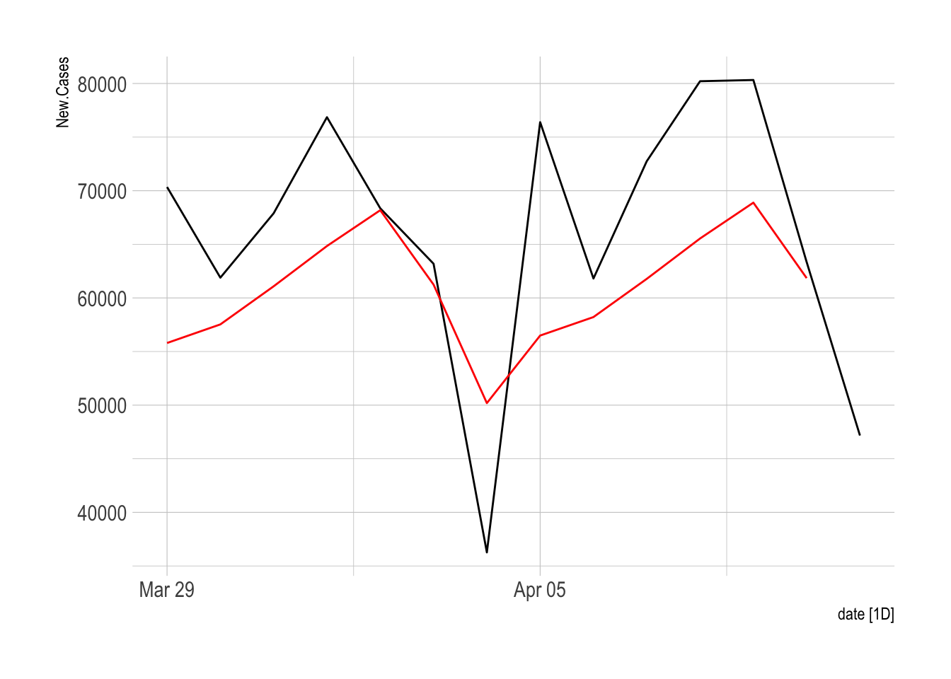
Full Future Forecast
First, I need to convert the entire original dataset and reestimate the model using all the data.
NCases <- NYTAgg.COVID %>%
    filter(is_aggregated(state)) %>%
    select(New.Cases)
# Turn it into a time series.  Notice the axis is a mess
NCasesTS <- as.ts(NCases, frequency = 7)
NCasesTS
Time Series:
Start = 2020.24863387978
End = 2073.82006245121
Frequency = 7
[1] 26871 29673 32253 34952 25551 30875 30268 31634 34499 33395
[11] 31553 26999 25760 26667 29953 31504 31475 28339 25236 27352
[21] 25810 28772 33393 36676 34375 26669 23064 24635 26486 30284
[31] 33934 29290 26088 21893 23660 24461 28413 27520 24850 20292
[41] 17560 22256 21115 26864 26120 23610 18957 21763 20882 22998
[51] 25685 23682 22198 19941 19029 18828 18670 22422 24387 23325
[61] 20573 21800 20726 19897 21127 28597 22221 18545 18144 18663
[71] 22708 23176 25308 25179 19008 20037 24824 25601 27945 30745
[81] 31733 26317 30427 34934 36846 41101 45480 42155 39385 39425
[91] 48164 49889 55473 57059 49899 44638 46630 53947 59398 59761
[101] 67937 60474 57492 61200 65460 68079 75476 70357 62103 61665
[111] 59475 64789 69610 69563 73016 66201 53605 58870 62704 66549
[121] 68432 68856 55717 50254 47076 52985 53344 57201 60385 54500
[131] 47764 46437 52696 53592 53596 58739 50176 41819 36691 42224
[141] 42738 45674 48172 44295 31990 39528 38972 45159 44814 45904
[151] 43992 33127 36021 43770 31814 46127 52002 41933 29996 24314
[161] 28717 33278 37196 47249 38573 33055 36451 38745 39109 44688
[171] 48022 40496 35499 54238 37219 41430 43992 53489 42168 36407
[181] 36241 42495 41724 46036 52833 47068 34842 61649 42366 52935
[191] 55789 58309 51106 44454 47361 53989 58802 64694 70025 52511
[201] 47239 64565 59767 63968 74827 83262 78251 58451 73873 73940
[211] 81745 89363 98835 83758 73649 92499 91517 107909 120836 131643
[221] 124904 103233 129562 139286 142520 162213 180743 158372 134480 165770
[231] 160994 171833 186918 197928 170837 139702 178936 177488 180445 102349
[241] 204414 150210 136211 166960 183442 200753 217344 230854 204720 170942
[251] 203287 219147 219057 224677 278938 206697 183500 200523 202504 244756
[261] 237297 249808 192825 178709 201187 200584 227194 193156 100343 215832
[271] 151308 188624 198948 228879 230602 146483 290498 201729 251309 234500
[281] 255683 280009 298487 251520 207812 222668 228619 229115 238419 239778
[291] 201057 168597 142058 184571 186863 189910 191173 167111 128537 155148
[301] 151130 155467 164936 165224 133442 113279 139202 117632 119896 125498
[311] 129467 104707 86808 92477 96220 94808 105500 99240 84384 63545
[321] 55121 63919 70060 71781 77884 69523 54934 59283 71569 74049
[331] 77689 78027 62498 50666 56391 57634 66632 67247 65530 56338
[341] 39846 98365 55862 58373 62325 64005 49488 37832 56920 54374
[351] 58866 60524 60382 54305 33942 54427 56651 79645 69227 74344
[361] 60332 44306 70343 61890 67895 76856 68358 63188 36267 76390
[371] 61812 72750 80211 80326 63339 47167# Time for tbats
FFCNCTS <- tbats(NCasesTS, use.box.cox = TRUE, seasonal.periods = 7)
# The tbats result
FFCNCTSTBATS(0, {0,0}, 0.945, {<7,3>})
Call: tbats(y = NCasesTS, use.box.cox = TRUE, seasonal.periods = 7)
Parameters
Lambda: 0
Alpha: 0.3269996
Beta: 0.03868864
Damping Parameter: 0.945277
Gamma-1 Values: 0.001335585
Gamma-2 Values: 0.001444268
Seed States:
[,1]
[1,] 10.352381486
[2,] -0.002115699
[3,] 0.055937556
[4,] -0.045746150
[5,] 0.018518612
[6,] 0.103836537
[7,] -0.036220228
[8,] 0.031873846
attr(,"lambda")
[1] 0.00000005919664
Sigma: 0.1283412
AIC: 9015.018Full Data Estimates
Now let me forecast that.
TBATS.FFC <- forecast(FFCNCTS, h = 14) %>%
    as_tibble() %>%
    mutate(Forecast = `Point Forecast`, date = as.Date("2021-04-12") + days(0:13)) %>%
    as_tsibble(index = date)
autoplot(NYTAgg.COVID %>%
    filter(is_aggregated(state)) %>%
    select(New.Cases)) + autolayer(TBATS.FFC %>%
    select(Forecast), color = "red") + labs(title = "Future Forecast for US COVID-19 Cases") +
    theme_ipsum_rc()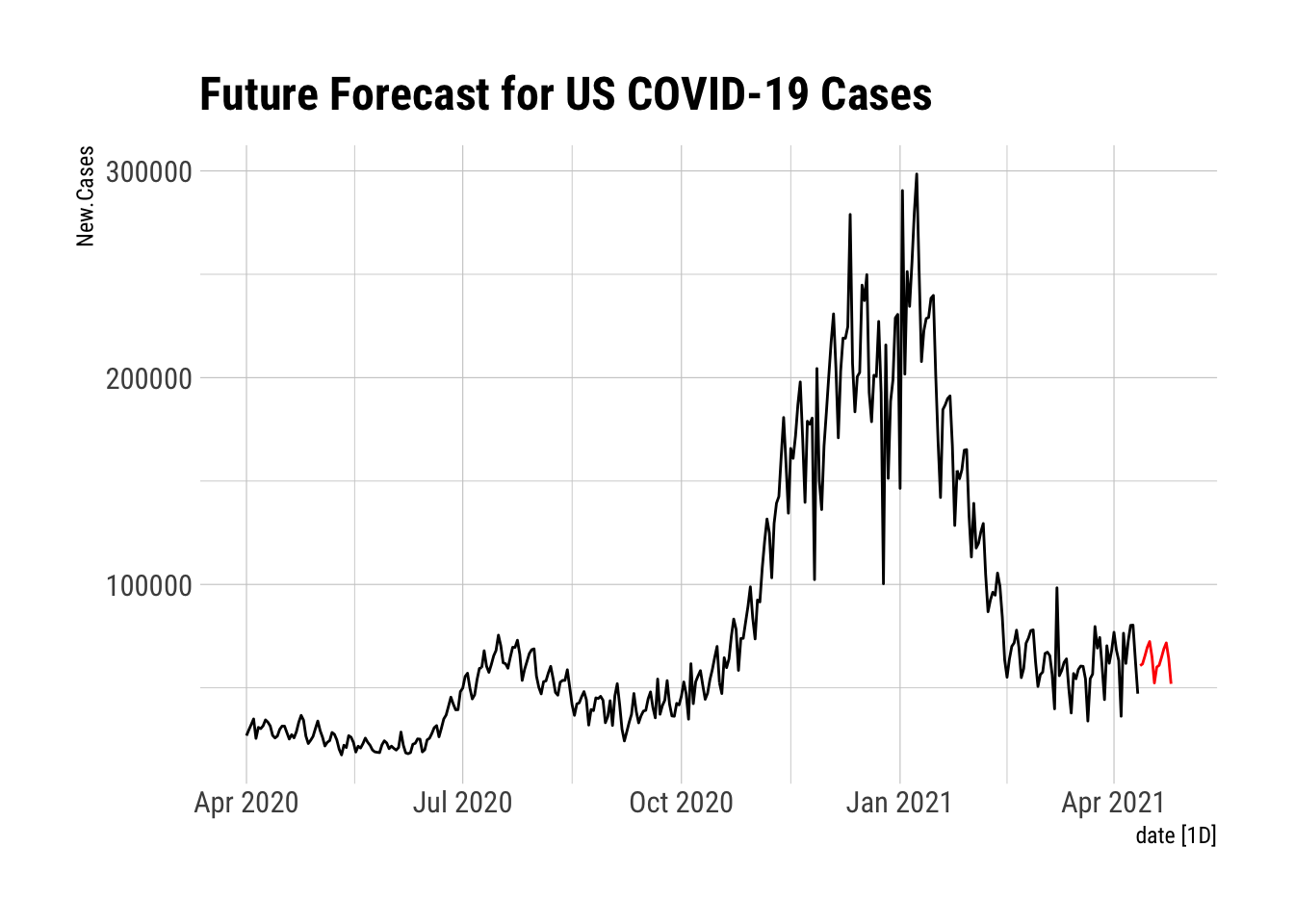
New Deaths
# To use tbats, I need an old style time series First, select the data of
# interest: New.Cases and make it match up with the training set
NDT <- COVID.Agg.Train %>%
    filter(is_aggregated(state)) %>%
    select(New.Deaths)
# Turn it into a time series.  Notice the axis is a mess
NDTS <- as.ts(NDT, frequency = 7)
NDTS
Time Series:
Start = 2020.24863387978
End = 2071.82006245121
Frequency = 7
[1] 1016 1215 1387 1553 1366 1524 2231 2084 2111 2257 2080 1679 1762 2705 2746
[16] 2343 2286 1949 1539 1836 2671 2368 2146 2124 1960 1252 1442 2392 2514 2204
[31] 1760 1582 1329 1089 2232 2708 1955 1570 1453 928 979 1651 1767 1736 1588
[46] 1225 843 845 1520 1476 1310 1288 1049 620 508 747 1485 1198 1189 962
[61] 601 734 1080 987 1008 1111 727 390 722 1030 928 876 777 692 316
[76] 448 769 761 727 698 546 255 360 833 767 2464 633 510 270 347
[91] 1300 642 723 590 260 262 391 956 946 841 828 667 395 425 952
[106] 969 957 896 774 412 529 1127 1130 1113 1143 874 440 1696 1319 1393
[121] 1258 1424 1049 415 608 1349 1243 1059 1349 957 534 537 1443 1470 1202
[136] 1165 1047 508 535 1338 1285 1030 1154 943 436 502 1206 1182 1118 997
[151] 867 368 487 1087 1068 1072 972 702 396 261 451 1156 902 1214 688
[166] 395 444 1270 978 829 935 663 210 428 935 1086 874 844 762 265
[181] 345 912 965 843 856 700 327 417 720 985 917 910 583 416 346
[196] 822 1005 791 874 675 382 512 928 1201 818 922 867 332 530 979
[211] 1012 1001 961 836 418 533 1125 1604 1103 1236 1007 454 733 1456 1419
[226] 1164 1384 1203 609 783 1596 1904 1949 1946 1404 835 1023 2202 2297 1159
[241] 1404 1185 807 1258 2592 2864 2845 2619 2178 1104 1523 2818 3142 2920 2944
[256] 2236 1350 1667 3013 3593 3287 2860 2552 1403 1948 3230 3395 2808 1120 1646
[271] 1217 1888 3624 3784 3442 1902 2367 1332 2039 3682 3956 4093 3890 3237 1763
[286] 2036 4402 3916 3960 3735 3329 1729 1440 2771 4366 4120 3702 3312 1813 1901
[301] 4092 4092 3861 3589 2630 1858 1943 3601 3836 5109 3564 2657 1290 1577 3165
[316] 3250 3872 5458 3364 1077 993 1703 2465 2615 2614 1821 1225 1450 2325 3189
[331] 2456 2169 1558 1124 1424 1303 2361 1944 2480 1454 676 814 1884 1473 1520
[346] 1703 1846 569 749 1243 1175 1554 1510 769 444 648 890 1588 1267 1256
[361] 777 487Estimate
# Time for tbats
FCNDTS <- tbats(NDTS)
# The tbats result
FCNDTS
TBATS(0.186, {2,2}, 0.905, {<7,3>})
Call: tbats(y = NDTS)
Parameters
Lambda: 0.185872
Alpha: -0.01027017
Beta: 0.02869088
Damping Parameter: 0.905439
Gamma-1 Values: 0.0009337819
Gamma-2 Values: -0.0004006507
AR coefficients: -0.136387 0.362833
MA coefficients: 0.557124 -0.100951
Seed States:
[,1]
[1,] 14.820902020
[2,] 0.465771739
[3,] 1.305662745
[4,] 0.006040356
[5,] -0.110715562
[6,] 0.877253118
[7,] -0.723397334
[8,] 0.096204317
[9,] 0.000000000
[10,] 0.000000000
[11,] 0.000000000
[12,] 0.000000000
attr(,"lambda")
[1] 0.1858719
Sigma: 0.7859871
AIC: 6189.533Compare Models
The following code chunk is not executed but was the basis for the set of results to compare. Key to this, they are estimated on the same data.
lambdaD <- NYTAgg.COVID %>%
    filter(is_aggregated(state)) %>%
    features(New.Deaths, features = guerrero) %>%
    pull(lambda_guerrero)
COVID.Models.KD <- COVID.Agg.Train %>%
    filter(is_aggregated(state)) %>%
    model(`K = 1` = ARIMA(box_cox(New.Deaths, lambdaD) ~ fourier(K = 1)), `K = 2` = ARIMA(box_cox(New.Deaths,
        lambdaD) ~ fourier(K = 2)), `K = 3` = ARIMA(box_cox(New.Deaths, lambdaD) ~
        fourier(K = 3)), `DK = 1` = ARIMA(New.Deaths ~ fourier(K = 1)), `DK = 2` = ARIMA(New.Deaths ~
        fourier(K = 2)), `DK = 3` = ARIMA(New.Deaths ~ fourier(K = 3)))
COVID.Models.KD %>%
    glance()
# A tibble: 6 x 9
state .model sigma2 log_lik AIC AICc BIC ar_roots ma_roots
<chr*> <chr> <dbl> <dbl> <dbl> <dbl> <dbl> <list> <list>
1 <aggregated> K = 1 0.284 -284. 581. 582. 609. <cpl [15]> <cpl [1]>
2 <aggregated> K = 2 0.249 -258. 534. 534. 569. <cpl [7]> <cpl [9]>
3 <aggregated> K = 3 0.242 -251. 527. 529. 578. <cpl [10]> <cpl [2]>
4 <aggregated> DK = 1 133786. -2641. 5299. 5299. 5330. <cpl [15]> <cpl [8]>
5 <aggregated> DK = 2 128733. -2632. 5286. 5286. 5328. <cpl [3]> <cpl [3]>
6 <aggregated> DK = 3 127890. -2630. 5285. 5286. 5336. <cpl [3]> <cpl [3]>Estimate the broad set of models.
COVID.Models.D <- COVID.Agg.Train %>%
    model(`K = 2` = ARIMA(box_cox(New.Deaths, lambdaD) ~ fourier(K = 2)), ARIMA = ARIMA(box_cox(New.Deaths,
        lambdaD)), ETS = ETS(box_cox(New.Deaths, lambdaD)), NNET = NNETAR(box_cox(New.Deaths,
        lambdaD))) %>%
    mutate(Combo1 = (`K = 2` + ARIMA + ETS)/3, Combo2 = (`K = 2` + ARIMA + ETS +
        NNET)/4) %>%
    reconcile(buARIMA = bottom_up(ARIMA), buK2 = bottom_up(`K = 2`), buETS = bottom_up(ETS))
How well does the ARIMA fit?
COVID.Models.D %>%
    filter(is_aggregated(state)) %>%
    select(ARIMA) %>%
    report()
Series: New.Deaths
Model: ARIMA(2,0,2)(1,1,1)[7]
Transformation: box_cox(New.Deaths, lambdaD)
Coefficients:
ar1 ar2 ma1 ma2 sar1 sma1
1.2312 -0.2401 -0.7756 0.0044 0.1865 -0.9242
s.e. 0.2543 0.2508 0.2573 0.1752 0.0747 0.0558
sigma^2 estimated as 0.2557: log likelihood=-263.57
AIC=541.13 AICc=541.46 BIC=568.24How about the ETS?
COVID.Models.D %>%
    filter(is_aggregated(state)) %>%
    select(ETS) %>%
    report()
Series: New.Deaths
Model: ETS(A,Ad,A)
Transformation: box_cox(New.Deaths, lambdaD)
Smoothing parameters:
alpha = 0.2770834
beta = 0.001578105
gamma = 0.1239983
phi = 0.8000154
Initial states:
l b s1 s2 s3 s4 s5
10.25626 0.6155904 0.5971836 -0.6575478 -0.8385621 -0.1883803 0.1239997
s6 s7
0.4877874 0.4755194
sigma^2: 0.2645
AIC AICc BIC
1665.132 1666.178 1715.723 Though the ARIMA model is much better, let me complete the TBATS exercise for this.
Forecast and Forecast Evaluation
# For comparison, the ARIMA model has AIC of 8012.8 so this is not an
# improvement; ; the ETS is 8645
TBATS.DFC <- forecast(FCNDTS, h = 13) %>%
    as_tibble() %>%
    select(`Point Forecast`) %>%
    tibble() %>%
    mutate(fperiod = row_number())
# Generate the forecast
COVID.Agg.Test %>%
    filter(is_aggregated(state)) %>%
    mutate(fperiod = row_number()) %>%
    left_join(TBATS.DFC) %>%
    mutate(MAE = mean(abs(New.Deaths - `Point Forecast`), na.rm = TRUE)) %>%
    head()
# A tsibble: 6 x 7 [1D]
# Key: state [1]
date state New.Cases New.Deaths fperiod `Point Forecast` MAE
<date> <chr*> <int> <int> <int> <dbl> <dbl>
1 2021-03-29 <aggregated> 70343 685 1 574. 172.
2 2021-03-30 <aggregated> 61890 947 2 1085. 172.
3 2021-03-31 <aggregated> 67895 1133 3 1164. 172.
4 2021-04-01 <aggregated> 76856 952 4 1058. 172.
5 2021-04-02 <aggregated> 68358 954 5 988. 172.
6 2021-04-03 <aggregated> 63188 748 6 765. 172.# Plot the forecast
COVID.Agg.Test %>%
filter(is_aggregated(state)) %>%
mutate(fperiod = row_number()) %>%
left_join(TBATS.DFC) %>%
autoplot(New.Deaths) + geom_line(aes(x = date, y = `Point Forecast`), color = "red") +
hrbrthemes::theme_ipsum() + labs(title = "Forecast New Deaths from COVID-19 and Actuals")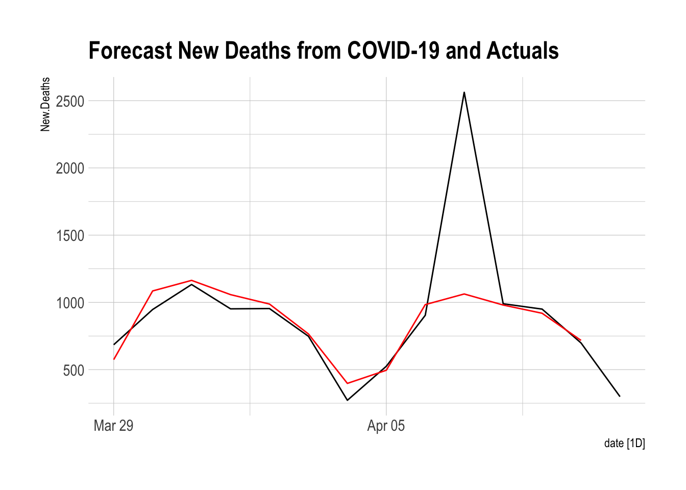
Full Future Forecast
First, I need to convert the entire original dataset and reestimate the model using all the data.
NDeaths <- NYTAgg.COVID %>%
    filter(is_aggregated(state)) %>%
    select(New.Deaths)
# Turn it into a time series.  Notice the axis is a mess
NDeathsTS <- as.ts(NDeaths, frequency = 7)
NDeathsTS
Time Series:
Start = 2020.24863387978
End = 2073.82006245121
Frequency = 7
[1] 1016 1215 1387 1553 1366 1524 2231 2084 2111 2257 2080 1679 1762 2705 2746
[16] 2343 2286 1949 1539 1836 2671 2368 2146 2124 1960 1252 1442 2392 2514 2204
[31] 1760 1582 1329 1089 2232 2708 1955 1570 1453 928 979 1651 1767 1736 1588
[46] 1225 843 845 1520 1476 1310 1288 1049 620 508 747 1485 1198 1189 962
[61] 601 734 1080 987 1008 1111 727 390 722 1030 928 876 777 692 316
[76] 448 769 761 727 698 546 255 360 833 767 2464 633 510 270 347
[91] 1300 642 723 590 260 262 391 956 946 841 828 667 395 425 952
[106] 969 957 896 774 412 529 1127 1130 1113 1143 874 440 1696 1319 1393
[121] 1258 1424 1049 415 608 1349 1243 1059 1349 957 534 537 1443 1470 1202
[136] 1165 1047 508 535 1338 1285 1030 1154 943 436 502 1206 1182 1118 997
[151] 867 368 487 1087 1068 1072 972 702 396 261 451 1156 902 1214 688
[166] 395 444 1270 978 829 935 663 210 428 935 1086 874 844 762 265
[181] 345 912 965 843 856 700 327 417 720 985 917 910 583 416 346
[196] 822 1005 791 874 675 382 512 928 1201 818 922 867 332 530 979
[211] 1012 1001 961 836 418 533 1125 1604 1103 1236 1007 454 733 1456 1419
[226] 1164 1384 1203 609 783 1596 1904 1949 1946 1404 835 1023 2202 2297 1159
[241] 1404 1185 807 1258 2592 2864 2845 2619 2178 1104 1523 2818 3142 2920 2944
[256] 2236 1350 1667 3013 3593 3287 2860 2552 1403 1948 3230 3395 2808 1120 1646
[271] 1217 1888 3624 3784 3442 1902 2367 1332 2039 3682 3956 4093 3890 3237 1763
[286] 2036 4402 3916 3960 3735 3329 1729 1440 2771 4366 4120 3702 3312 1813 1901
[301] 4092 4092 3861 3589 2630 1858 1943 3601 3836 5109 3564 2657 1290 1577 3165
[316] 3250 3872 5458 3364 1077 993 1703 2465 2615 2614 1821 1225 1450 2325 3189
[331] 2456 2169 1558 1124 1424 1303 2361 1944 2480 1454 676 814 1884 1473 1520
[346] 1703 1846 569 749 1243 1175 1554 1510 769 444 648 890 1588 1267 1256
[361] 777 487 685 947 1133 952 954 748 272 525 904 2562 990 950 698
[376] 299# Time for tbats
FFCNDTS <- tbats(NDeathsTS, use.box.cox = TRUE, seasonal.periods = 7)
# The tbats result
FFCNDTSTBATS(0.249, {0,0}, 0.902, {<7,2>})
Call: tbats(y = NDeathsTS, use.box.cox = TRUE, seasonal.periods = 7)
Parameters
Lambda: 0.248657
Alpha: 0.1989825
Beta: 0.02448758
Damping Parameter: 0.90166
Gamma-1 Values: 0.03913841
Gamma-2 Values: 0.0006746063
Seed States:
[,1]
[1,] 19.57619964
[2,] 0.55615064
[3,] 1.59565597
[4,] 0.01757539
[5,] 1.03842572
[6,] -0.82638433
attr(,"lambda")
[1] 0.2486569
Sigma: 1.278158
AIC: 6442.452Full Data Estimates
Now let me forecast that.
TBATS.DFFC <- forecast(FFCNDTS, h = 14) %>%
    as_tibble() %>%
    mutate(Forecast = `Point Forecast`, date = as.Date("2021-04-12") + days(0:13)) %>%
    as_tsibble(index = date)
autoplot(NYTAgg.COVID %>%
    filter(is_aggregated(state)) %>%
    select(New.Deaths)) + autolayer(TBATS.DFFC %>%
    select(Forecast), color = "red") + labs(title = "Future Forecast for US COVID-19 Deaths") +
    theme_ipsum_rc()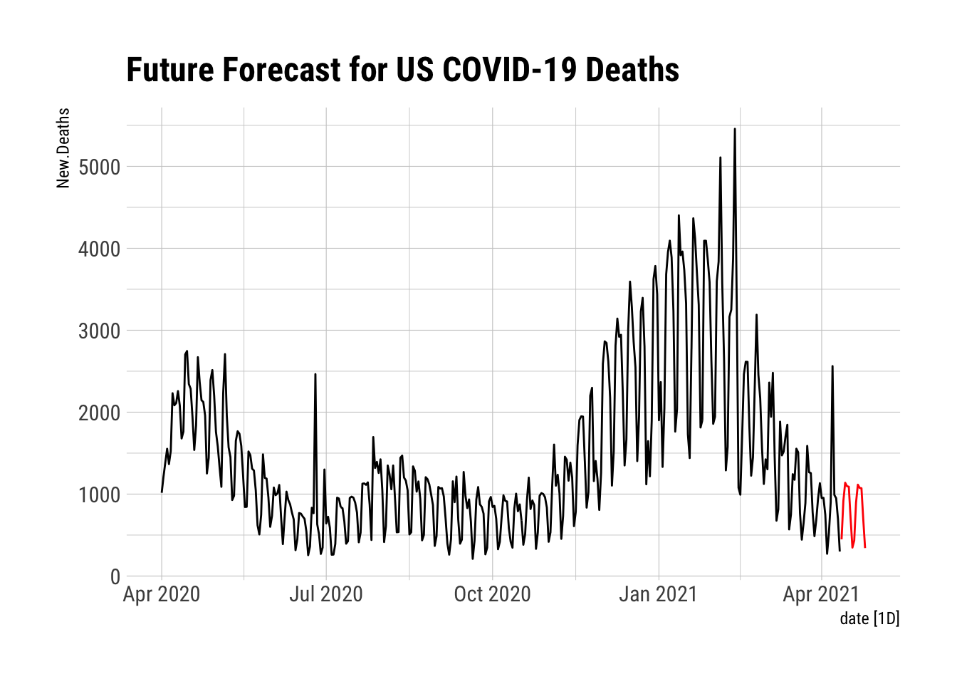
That looks much better than the recent data. I hope it is correct.
Robert W. Walker
Associate Professor of Quantitative Methods
My research interests include causal inference, statistical computation and data visualization.