Forecasting the Weather
Loading NWS Data
Load the data.
# There is one blank variable name and some garbage at the top.  Skip the first
# six rows and label M and - as missing.
NWS <- read.csv(url("https://www.weather.gov/source/pqr/climate/webdata/Portland_dailyclimatedata.csv"),
    skip = 6, na.strings = c("M", "-")) %>%
    rename(Variable = X)
One thing that will prove troublesome is that /A appears in a few places. I want to remove it. I will ask R to find all of the character columns and remove /A.
NWS <- NWS %>%
    mutate(across(where(is.character), ~str_remove(.x, "/A")))
First, let’s work on a monthly time series. Because the sum or average is already a column, I do not need to create it; I only need select it.
# Now to create a Monthly time series.
NWS.Monthly.Base <- NWS %>%
    select(YR, MO, Variable, AVG.or.Total)
Let me first fix the character values. There is only two character values remaining; there is 1 blank and some T values. From there, I will use pivot_wider to move variables to columns; create the time index, and turn the variables into numeric types.
NWS.Monthly.Tidy <- NWS.Monthly.Base %>%
    filter(!(MO == 1 & YR == 2020)) %>%
    filter(!(MO == 10 & YR == 1940)) %>%
    mutate(AVG.or.Total = recode(AVG.or.Total, T = "O.005")) %>%
    pivot_wider(., names_from = "Variable", values_from = "AVG.or.Total") %>%
    mutate(Month.Yr = yearmonth(paste(YR, MO, sep = "-"))) %>%
    mutate(TX = as.numeric(TX), TN = as.numeric(TN), PR = as.numeric(PR), SN = as.numeric(SN))
str(NWS.Monthly.Tidy)
tibble[,7] [950 × 7] (S3: tbl_df/tbl/data.frame)
$ YR : int [1:950] 1940 1940 1941 1941 1941 1941 1941 1941 1941 1941 ...
$ MO : int [1:950] 11 12 1 2 3 4 5 6 7 8 ...
$ TX : num [1:950] 49.1 48.5 47.4 55.1 63.5 65.8 67.1 71.6 84.5 77.6 ...
$ TN : num [1:950] 35.9 36 35.2 37.1 40.6 43.1 48.1 52.6 58.3 58 ...
$ PR : num [1:950] 4.53 4.85 5.27 1.59 1.74 1.66 4.27 0.81 0.03 1.45 ...
$ SN : num [1:950] 0 0 0 0 0 0 0 0 0 0 ...
$ Month.Yr: mth [1:950] 1940 Nov, 1940 Dec, 1941 Jan, 1941 Feb, 1941 Mar, 1941 Apr...head(NWS.Monthly.Tidy)# A tibble: 6 x 7
YR MO TX TN PR SN Month.Yr
<int> <int> <dbl> <dbl> <dbl> <dbl> <mth>
1 1940 11 49.1 35.9 4.53 0 1940 Nov
2 1940 12 48.5 36 4.85 0 1940 Dec
3 1941 1 47.4 35.2 5.27 0 1941 Jan
4 1941 2 55.1 37.1 1.59 0 1941 Feb
5 1941 3 63.5 40.6 1.74 0 1941 Mar
6 1941 4 65.8 43.1 1.66 0 1941 AprWell, that’s annoying. Some of the missingness here is a characteristic of the columns. Let’s see if we can do better at the end of the creation of the daily data.
NWS.Daily <- NWS %>%
    select(-AVG.or.Total)
names(NWS.Daily) <- c("YR", "MO", "Variable", paste0("Day.", 1:31))
NWS.Daily <- NWS.Daily %>%
    pivot_longer(., cols = starts_with("Day."), names_to = "Day", values_to = "value") %>%
    mutate(Day = str_remove(Day, "Day.")) %>%
    pivot_wider(., names_from = "Variable", values_from = "value") %>%
    mutate(PR = recode(PR, T = "O.005"), SN = recode(SN, T = "O.005")) %>%
    mutate(TX = as.numeric(TX), TN = as.numeric(TN), PR = as.numeric(PR), SN = as.numeric(SN),
        date = as.Date(paste(MO, Day, YR, sep = "-"), format = "%m-%d-%Y"))
NWS.Daily.Clean <- NWS.Daily %>%
    filter(!(is.na(date)))
A Backward Approach to the Monthly
NWS.Monthly.Sum <- NWS.Daily.Clean %>%
    group_by(MO, YR) %>%
    summarise(MaxAvg = mean(TX, na.rm = TRUE), MinAvg = mean(TN, na.rm = TRUE), Precip = sum(PR,
        na.rm = TRUE), Snow = sum(SN, na.rm = TRUE)) %>%
    ungroup() %>%
    mutate(Month = yearmonth(paste(YR, MO, sep = "-"))) %>%
    as_tsibble(., index = Month) %>%
    filter(year(Month) < 2020)
Plot the Monthly
NWS.Monthly.Sum %>%
    pivot_longer(cols = c(MaxAvg, MinAvg, Precip, Snow), names_to = "Type") %>%
    ggplot() + aes(x = Month, y = value) + geom_line() + facet_wrap(vars(Type), scales = "free_y")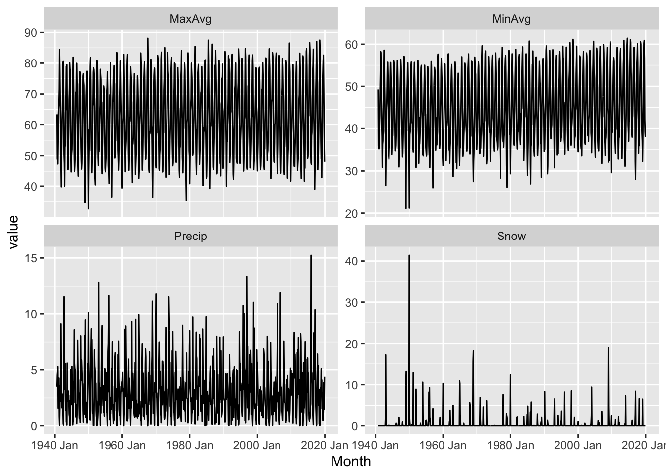
Monthly Decompositions
Decompose.Me <- function(data, var, trendW = 5, seasonW = 5) {
    var <- ensym(var)
    data %>%
        model(STL(!!var ~ trend(window = trendW) + season(window = seasonW))) %>%
        components() %>%
        autoplot()
}
Decompose.Me(NWS.Monthly.Sum, MaxAvg, trendW = 12)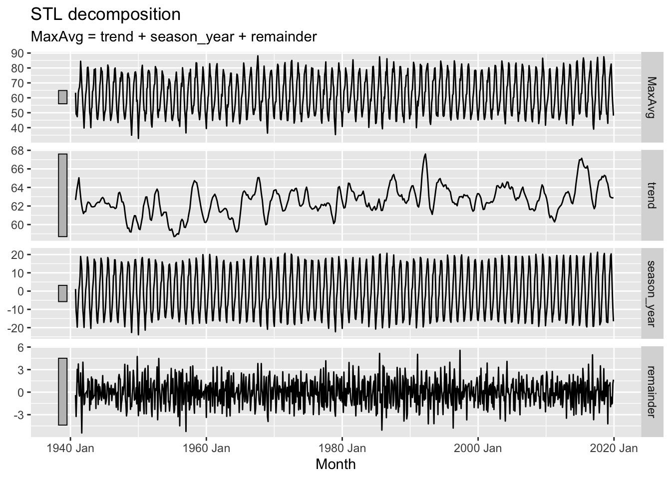
To work with the STL seasonally adjusted data, we can isolate season_adjust. This is the core component in STL+…
Let me decompose each series.
Decompose.Me(NWS.Monthly.Sum, MinAvg, trendW = 12)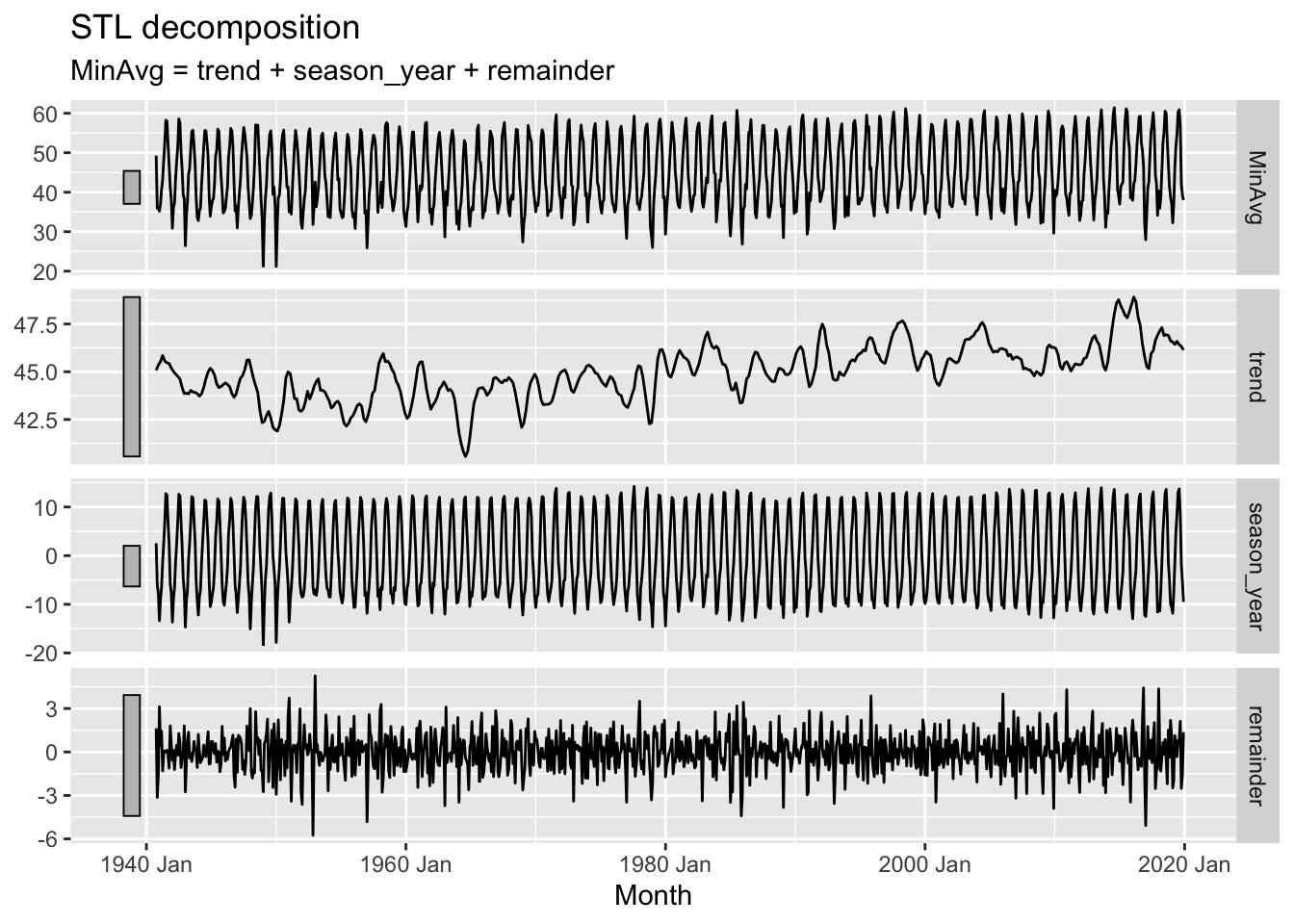
Cmp <- NWS.Monthly.Sum %>%
model(STL(MaxAvg ~ trend() + season())) %>%
components()
Cmp %>%
ggplot(.) + aes(x = Month, y = season_adjust) + geom_line(alpha = 0.2) + geom_point(aes(y = MaxAvg),
color = "red", alpha = 0.1)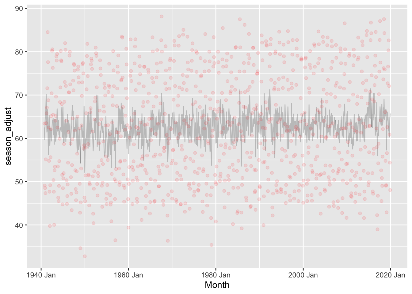 ### Precipitation
Decompose.Me(NWS.Monthly.Sum, Precip, trendW = 12)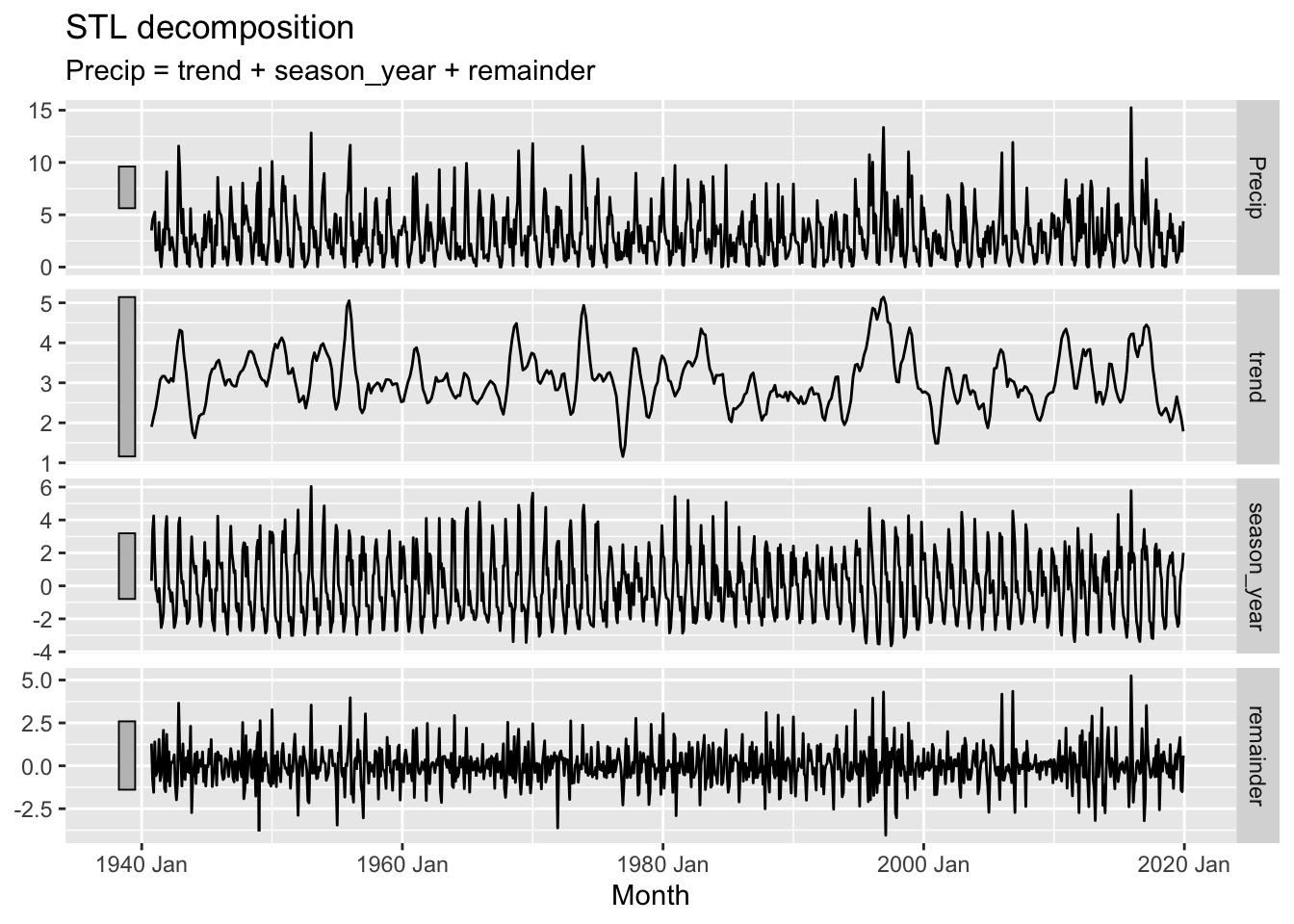
Snow
Decompose.Me(NWS.Monthly.Sum, Snow, trendW = 12)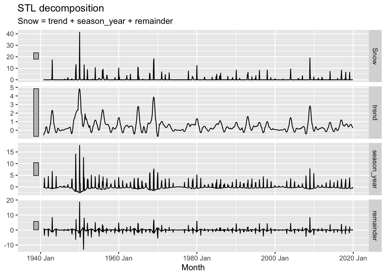
Training and Testing
That gives me the data that I want; now let me slice it up into training and test sets.
NWS.Monthly.Train <- NWS.Monthly.Sum %>%
    filter(YR < 2019)
NWS.Monthly.Test <- NWS.Monthly.Sum %>%
    anti_join(., NWS.Monthly.Train)
Model Fitting
Exploring a prophet.
Prophet
library(fable.prophet)
ProphMod <- NWS.Monthly.Train %>%
    model(prophet = prophet(MaxAvg ~ growth() + season("year", 12)))
PMF <- ProphMod %>%
    forecast(h = 12)
What does it look like?
Plot it
PMF %>%
    autoplot(alpha = 0.2) + geom_point(data = NWS.Monthly.Sum %>%
    filter(YR > 2016) %>%
    select(Month, MaxAvg), aes(x = Month, y = MaxAvg)) + geom_line(data = NWS.Monthly.Sum %>%
    filter(YR > 2016) %>%
    select(Month, MaxAvg), aes(x = Month, y = MaxAvg), alpha = 0.2) + labs(x = "Date",
    y = "Monthly Max Temp.", title = "Temp Forecast Using Prophet")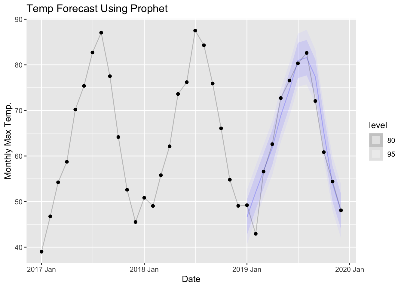
Some Models
I am going to define a little function that takes two inputs and analyses the set of models that I will want for each of them. The first input is the data. The second input is the name of the variable. There is a little programming trick here to allow us to pass that unquoted using ensym(). As an example, if I ask for Usual.Suspects(data=NWS.Monthly.Sum, MaxAvg) I would get all of these models applied to MaxAvg as a column in that dataset.
Usual.Suspects <- function(data, Outcome) {
    Outcome <- ensym(Outcome)
    fits <- data %>%
        model(`K = 1` = ARIMA(!!Outcome ~ fourier(K = 1)), `K = 2` = ARIMA(!!Outcome ~
            fourier(K = 2)), `K = 3` = ARIMA(!!Outcome ~ fourier(K = 3)), ARIMA = ARIMA(!!Outcome),
            ETS = ETS(!!Outcome), NNET = NNETAR(!!Outcome ~ fourier(K = 2)), prophet = prophet(!!Outcome ~
                growth() + season("year", 12))) %>%
        mutate(Combo1 = (`K = 2` + ARIMA + ETS)/3, Combo2 = (`K = 2` + ARIMA + ETS +
            NNET)/4)
    return(fits)
}
Execute it using pipes for the data.
MaxAvg <- NWS.Monthly.Train %>%
    Usual.Suspects(., Outcome = MaxAvg)
Actually forecasting it takes some time. I will only want to do that once so let me store it as an object.
MaxAFC <- MaxAvg %>%
    forecast(h = 12)
Assess the accuracy of the forecast, here over 12 periods.
MaxAFC %>%
    accuracy(NWS.Monthly.Test)
# A tibble: 8 x 10
.model .type ME RMSE MAE MPE MAPE MASE RMSSE ACF1
<chr> <chr> <dbl> <dbl> <dbl> <dbl> <dbl> <dbl> <dbl> <dbl>
1 ARIMA Test -1.17 3.12 2.55 -1.78 4.21 NaN NaN 0.0456
2 Combo1 Test -1.25 3.24 2.26 -2.31 3.95 NaN NaN -0.0820
3 Combo2 Test -1.06 3.17 2.23 -2.06 3.95 NaN NaN -0.0881
4 ETS Test -1.64 3.79 2.56 -3.15 4.56 NaN NaN -0.0868
5 K = 1 Test -0.377 2.65 2.17 -1.03 3.84 NaN NaN -0.234
6 K = 2 Test -0.944 3.32 2.23 -2.00 3.98 NaN NaN -0.00881
7 K = 3 Test -0.945 3.35 2.25 -2.00 4.01 NaN NaN -0.00952
8 NNET Test -0.507 3.31 2.26 -1.35 4.14 NaN NaN 0.0190 Pick and store the minimum.
Min.Model <- MaxAFC %>%
    accuracy(NWS.Monthly.Test) %>%
    slice_min(., order_by = MAE, n = 1)
Min.Model
# A tibble: 1 x 10
.model .type ME RMSE MAE MPE MAPE MASE RMSSE ACF1
<chr> <chr> <dbl> <dbl> <dbl> <dbl> <dbl> <dbl> <dbl> <dbl>
1 K = 1 Test -0.377 2.65 2.17 -1.03 3.84 NaN NaN -0.234Show the forecast for it.
MaxAFC %>%
    filter(.model == Min.Model$.model) %>%
    autoplot() + autolayer(NWS.Monthly.Sum %>%
    slice_max(., order_by = Month, n = 24) %>%
    select(MaxAvg)) + theme_ipsum_rc() + labs(title = "Winner Forecast of Max Avg. Temp. in Oregon")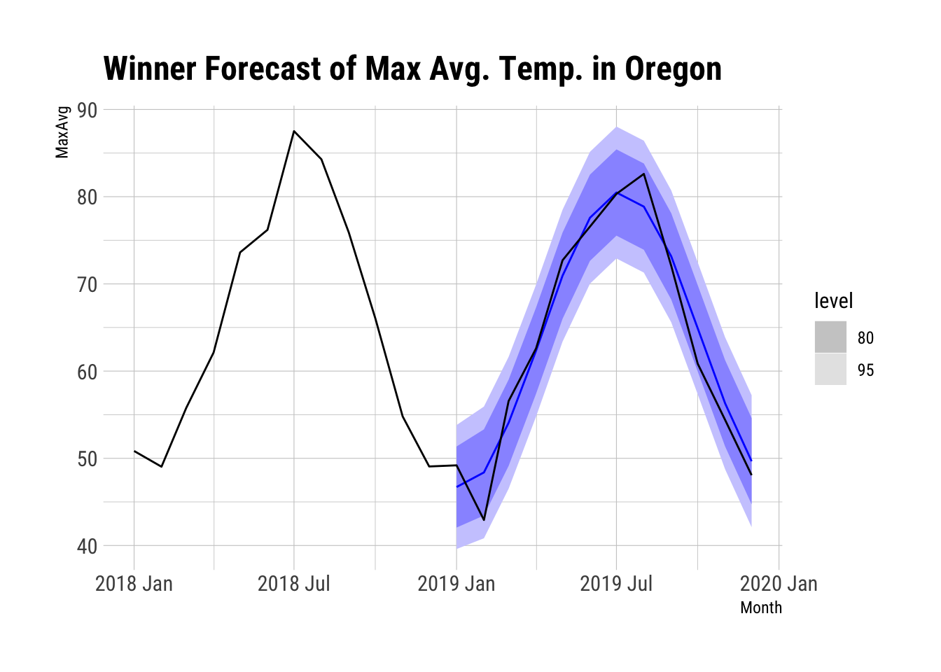
Automagics
I want to write a magic function. It takes four inputs: data, Outcome, DateVar, and H.Horizon [defaults to 12]. The first one is the data. The next two inputs are Outcome, the outcome without quotation marks, and DateVar – the Date variable [the index of the tsibble], also unquoted. The final argument sets the forecast horizon [the plots will have two times this before them in real data from the test set]. I have tried to be copious in commenting this.
A Monthly Forecast Function
Accuse.Usual.Suspect <- function(data, Outcome, DateVar, H.Horizon = 12) {
    # Turn the symbols -- names that will make sense in their environments when
    # called -- that the user supplies into symbolics.  This is the role of ensym.
    Outcome <- ensym(Outcome)
    DateVar <- ensym(DateVar)
    # Create test using H.Horizon
    test <- data %>%
        slice_max(., order_by = !!DateVar, n = H.Horizon)  # Create train
    train <- data %>%
        anti_join(., test)
    # Estimate some models and store them as fits.  !! calls the variable name in the
    # given environment
    fits <- train %>%
        Usual.Suspects(., !!Outcome)
    # Forecast the models
    FC <- fits %>%
        forecast(h = H.Horizon)
    # Compare train and test using accuracy
    Accuracy.Table <- FC %>%
        accuracy(test)
    # Show the best fit
    Min.Model <- Accuracy.Table %>%
        slice_min(., order_by = MAE, n = 1)
    # Report on the best fitting model
    Min.Report <- fits %>%
        select(Min.Model$.model) %>%
        report()
    # Create a plot of the time series residuals for the best fit
    Min.Res.Plot <- fits %>%
        select(Min.Model$.model) %>%
        gg_tsresiduals()
    # Create a forecast plot for the best fitting model.
    Min.ForeCPlot <- FC %>%
        filter(.model == Min.Model$.model) %>%
        autoplot() + autolayer(test %>%
        select(!!Outcome)) + autolayer(data %>%
        slice_max(., order_by = !!DateVar, n = H.Horizon * 3) %>%
        select(!!Outcome)) + theme_ipsum_rc() + labs(title = "Winner Forecast")
    # Return a named list with all the stuff we calculated along the way.
    fit.list <- list(test = test, train = train, Model.Fits = fits, Model.Forecasts = FC,
        Accuracy.Table = Accuracy.Table, Min.Model = Min.Model, Min.Report = Min.Report,
        Min.Res.Plot = Min.Res.Plot, Min.Forecast.Plot = Min.ForeCPlot)
    return(fit.list)
}
Minimum Average Temperature
Try out the big function.
MinAvg.Res <- MinAvg.Res <- NWS.Monthly.Sum %>%
    Accuse.Usual.Suspect(., Outcome = MinAvg, DateVar = Month, H.Horizon = 14)
Series: MinAvg
Model: LM w/ ARIMA(2,1,2)(0,0,1)[12] errors
Coefficients:
ar1 ar2 ma1 ma2 sma1 fourier(K = 1)C1_12
0.5867 -0.1604 -1.3077 0.3216 0.1457 -11.1766
s.e. 0.1736 0.0503 0.1729 0.1701 0.0317 0.1583
fourier(K = 1)S1_12
-1.6573
s.e. 0.1581
sigma^2 estimated as 5.996: log likelihood=-2164.31
AIC=4344.62 AICc=4344.77 BIC=4383.35
Try out a result.
MinAvg.Res$Min.Forecast.Plot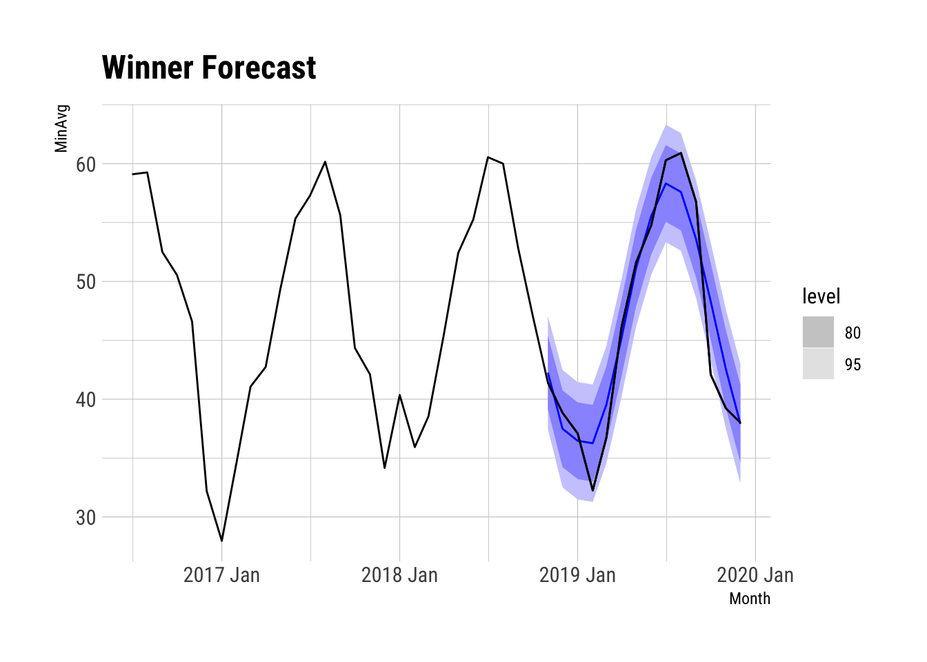
Precipitation
Try it with precipitation.
Precip.Res <- Accuse.Usual.Suspect(data = NWS.Monthly.Train, Outcome = Precip, DateVar = Month,
    H.Horizon = 12)
Series: Precip
Model: LM w/ ARIMA(0,0,1) errors
Coefficients:
ma1 fourier(K = 2)C1_12 fourier(K = 2)S1_12 fourier(K = 2)C2_12
0.1396 2.3157 -0.3704 -0.0789
s.e. 0.0319 0.0924 0.0923 0.0885
fourier(K = 2)S2_12 intercept
-0.7328 3.0929
s.e. 0.0885 0.0663
sigma^2 estimated as 3.155: log likelihood=-1844.89
AIC=3703.78 AICc=3703.9 BIC=3737.6
Forecast me.
Precip.Res$Min.Forecast.Plot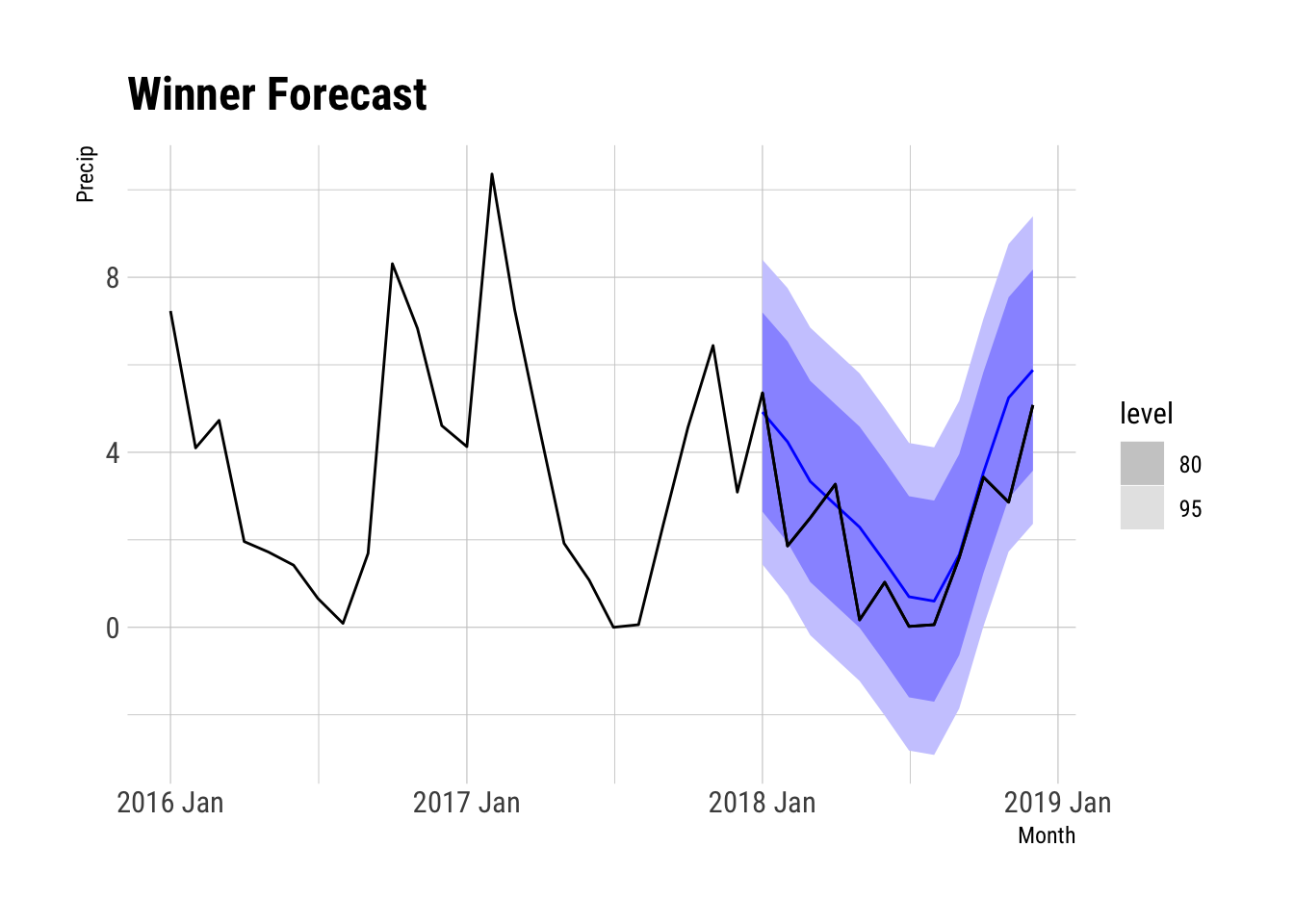
Snow
Snow.Res <- NWS.Monthly.Sum %>%
    Accuse.Usual.Suspect(., Outcome = MinAvg, DateVar = Month, H.Horizon = 18)
Series: MinAvg
Model: LM w/ ARIMA(3,1,2) errors
Coefficients:
ar1 ar2 ar3 ma1 ma2 fourier(K = 2)C1_12
0.9924 -0.1268 0.0006 -1.7788 0.7825 -11.1720
s.e. 0.0961 0.0493 0.0342 0.0903 0.0892 0.1218
fourier(K = 2)S1_12 fourier(K = 2)C2_12 fourier(K = 2)S2_12
-1.6619 0.8254 1.1861
s.e. 0.1217 0.1110 0.1110
sigma^2 estimated as 5.331: log likelihood=-2099.14
AIC=4218.27 AICc=4218.51 BIC=4266.65
THat should give me a monthly forecast for everything.
Now, what if I want to forecast that model into the future? If I wanted to include this in the original function, it would require estimating models that I do not need. So instead, here I know what model I need, say, for Precipitation, that would be:
Precip.Res$Min.Model# A tibble: 1 x 10
.model .type ME RMSE MAE MPE MAPE MASE RMSSE ACF1
<chr> <chr> <dbl> <dbl> <dbl> <dbl> <dbl> <dbl> <dbl> <dbl>
1 K = 2 Test -0.790 1.24 0.941 -486. 489. NaN NaN -0.394So estimate that model on the entire data and plot the forecast from it.
NWS.Monthly.Sum %>%
    model(K1 = ARIMA(Precip ~ fourier(K = 1) + PDQ(0, 0, 0))) %>%
    forecast(h = 12) %>%
    autoplot() + autolayer(NWS.Monthly.Sum %>%
    slice_max(., order_by = Month, n = 24)) + theme_ipsum_rc()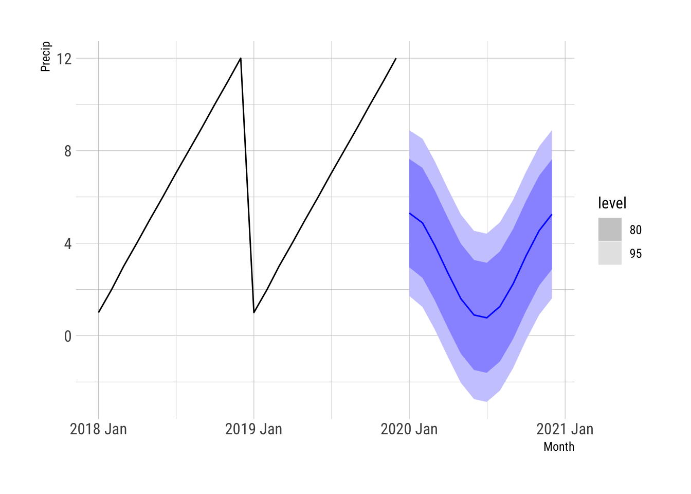
Robert W. Walker
Associate Professor of Quantitative Methods
My research interests include causal inference, statistical computation and data visualization.