Spurious Regressions
Regression Basics
A regression of two completely random variables, in this case normal, should result in about 5% of t-statistics with p-values less than 0.05. This is the basis for the interpretation of a p-value; how often would we see something this extreme or even more extreme randomly?
NReg <- function(junk) {
y1 <- rnorm(200)
y2 <- rnorm(200)
return(summary(lm(y1~y2))$coefficients[2,4])
}
NReg.Result <- data.frame(Res=sapply(1:1000, function(x) {NReg(x)}))
table(NReg.Result$Res < 0.05)
##
## FALSE TRUE
## 949 51Checks out.
Regressions of Cumulated Time Series
Spurious <- function(junk) {
y1 <- cumsum(rnorm(200))
y2 <- cumsum(rnorm(200))
return(summary(lm(y1~y2))$coefficients[2,4])
}
Spurious.Result <- data.frame(Res=sapply(1:1000, function(x) {Spurious(x)}))
Finally, let’s plot the p-values.
Spurious.Result %>% ggplot(., aes(x=Res)) + geom_histogram(bins=20)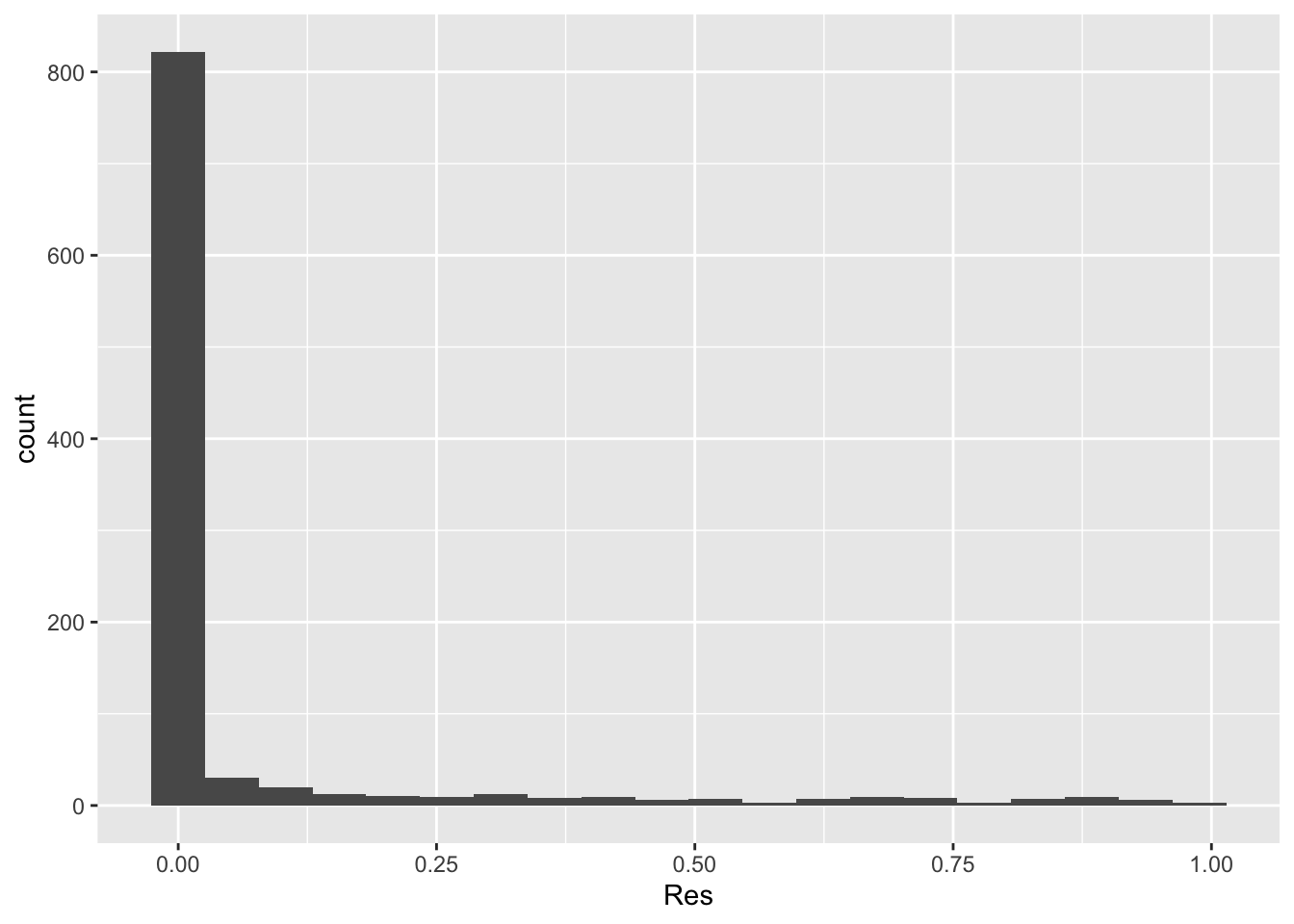
This is unexpected. Over 80% are less than 0.05. Let’s understand a bit of why. What does a series from each look like?
Example Series
par(mfrow=c(2,1))
plot(seq(1,1000), rnorm(1000), type="l")
plot(seq(1,1000), cumsum(rnorm(1000)), type="l")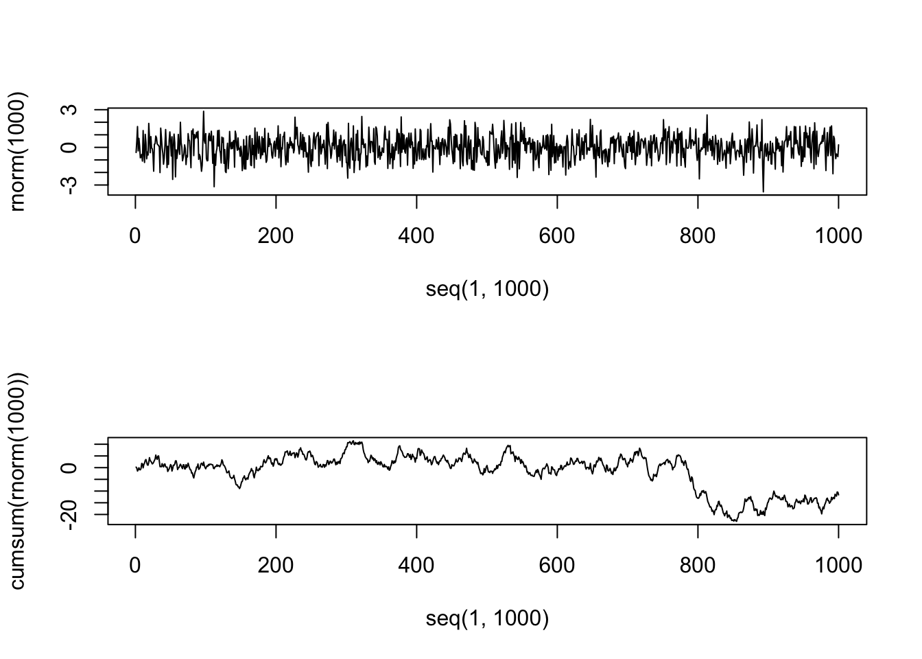
Robert W. Walker
Associate Professor of Quantitative Methods
My research interests include causal inference, statistical computation and data visualization.