I want to use a dataset from fpp3 and have a look at how the code translation works for the things that they do. The organizing form for the data is a little bit different among the two as fpp3 is built around the tsibble as construct while timetk dodges that with the use of a bit more explicit declarations. In many ways, as some of you have learned through frustration with aggregation and tsibble, this is more flexible because not all time is neatly embedded in all other time [weeks <=> months]. Let’s use US employment and focus in on the retail trade part since 1990.

library(fpp3)

## -- Attaching packages -------------------------------------------- fpp3 0.4.0 --

## v tibble      3.1.0      v tsibble     1.0.0 
## v dplyr       1.0.5      v tsibbledata 0.3.0 
## v tidyr       1.1.3      v feasts      0.2.1 
## v lubridate   1.7.10     v fable       0.3.0 
## v ggplot2     3.3.3

## -- Conflicts ------------------------------------------------- fpp3_conflicts --
## x lubridate::date()    masks base::date()
## x dplyr::filter()      masks stats::filter()
## x tsibble::intersect() masks base::intersect()
## x tsibble::interval()  masks lubridate::interval()
## x dplyr::lag()         masks stats::lag()
## x tsibble::setdiff()   masks base::setdiff()
## x tsibble::union()     masks base::union()

us_employment %>% filter(Title=="Retail Trade")

## # A tsibble: 969 x 4 [1M]
## # Key:       Series_ID [1]
##       Month Series_ID     Title        Employed
##       <mth> <chr>         <chr>           <dbl>
##  1 1939 Jan CEU4200000001 Retail Trade    3009 
##  2 1939 Feb CEU4200000001 Retail Trade    3002.
##  3 1939 Mar CEU4200000001 Retail Trade    3052.
##  4 1939 Apr CEU4200000001 Retail Trade    3098.
##  5 1939 May CEU4200000001 Retail Trade    3123 
##  6 1939 Jun CEU4200000001 Retail Trade    3141.
##  7 1939 Jul CEU4200000001 Retail Trade    3100 
##  8 1939 Aug CEU4200000001 Retail Trade    3092.
##  9 1939 Sep CEU4200000001 Retail Trade    3191.
## 10 1939 Oct CEU4200000001 Retail Trade    3242.
## # ... with 959 more rows

us_employment %>% filter(Title=="Retail Trade" & Month > yearmonth("1999-12") ) %>% autoplot()

## Plot variable not specified, automatically selected `.vars = Employed`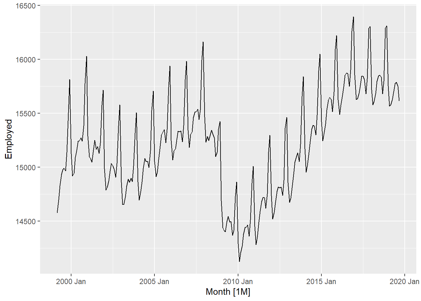

There’s the tsibble. Let me create my own version of the data to operate on.

my_usemp <- us_employment %>% filter(Title=="Retail Trade", Month > yearmonth("1999-12"))

timetk has a plotter that is very similar but we will need a proper date. If you set interactive to true and pass it, you get plotly by default. The key for making it work will be the deployment of a standard date format or something like it; the acceptable types are covered here.

library(timetk); library(magrittr)

## 
## Attaching package: 'magrittr'

## The following object is masked from 'package:tidyr':
## 
##     extract

my_usemp %<>% mutate(Date = as.Date(Month))
interactive <- TRUE
my_usemp %>% plot_time_series(Date, Employed, .interactive=interactive)

The plotly slider feature is particularly neat.

my_usemp %>% plot_time_series(Date, Employed, .interactive=interactive, .plotly_slider = TRUE)

my_usemp %>%plot_seasonal_diagnostics(Date, Employed, .interactive=interactive)

my_usemp %>% plot_stl_diagnostics(
        Date, Employed,
        .frequency = "auto", .trend = "auto",
        .feature_set = c("observed", "season", "trend", "remainder"),
        .interactive = interactive)

## frequency = 12 observations per 1 year

## trend = 60 observations per 5 years

my_usemp %>% plot_acf_diagnostics(
    Date, Employed,               # ACF & PACF
    .lags = "12 months")